12.1 Columnar organization
Before we turn, in Section 12.2, to the rather abstract notion of a ’neuronal population’, we present in this section a short introduction into the structural organization and functional characterization of cortex. We will argue that a cortical column, or more precisely, a group of cells consisting of neurons of the same type in one layer of a cortical column, can be considered as a plausible biological candidate of a neuronal population.
12.1.1 Receptive fields
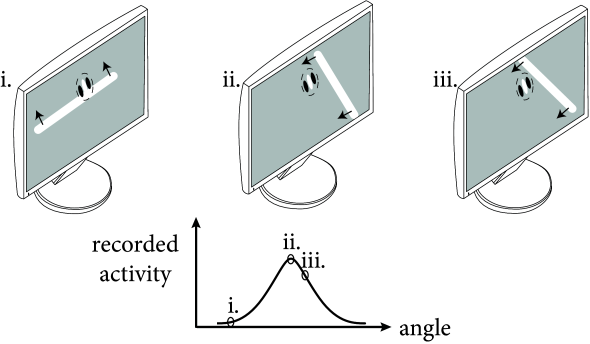
Neurons in sensory cortices can be experimentally characterized by the stimuli to which they exhibit a strong response. The receptive field of so-called simple cells in visual cortex (cf. Chapter 1) has typically two or three elongated spatial subfields. The neuron responds maximally to a moving light bar with an orientation aligned with the elongation of the positive subfield. If the orientation of the stimulus changes, the activity of the cell decreases (Fig. 12.3). Thus simple cells in visual cortex are sensitive to the orientation of a light bar (231).
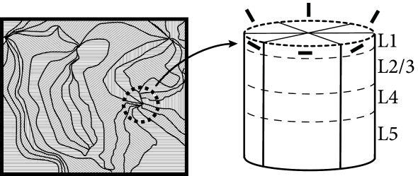
In this and the following chapters, we exploit the fact that neighboring neurons in visual cortex have similar receptive fields. If the experimentalist moves the electrode vertically down from the cortical surface to deeper layers, the location of the receptive field and its preferred orientation does not change substantially. If the electrode is moved to a neighboring location in cortex, the location and preferred orientation of the receptive field of neurons at the new location changes only slightly compared to the receptive fields at the previous location. This observation has led to the idea that cortical cells can be grouped into ‘columns’ of neurons with similar properties. Each column stretches across different cortical layers, but has only a limited extent on the cortical surface (231). The exact size and anatomical definition of a cortical column is a matter of debate, but each column is likely to contain several thousand neurons with similar receptive fields (310).
In other sensory cortices, the characterization of neuronal receptive fields is analogous to that in visual cortex. For example, in auditory cortex neurons can be characterized by stimulation with pure tunes. Each neuron has its preferred tone frequency and neighboring neurons have similar preferences. In the somatosensory cortex neurons that respond strongly to touch on, e.g., the index finger are located close to each other. The concepts of receptive field and optimal stimuli are not restricted to mammals or cortex, but are also routinely used in studies of, e.g., retinal ganglion cells, thalamic cells, olfactory bulb, or insect sensory systems.
Example: Cortical Maps
Neighboring neurons have similar receptive fields, but the exact characteristics of the receptive fields change slightly as one moves parallel to the cortical surface. This gives rise to cortical maps.
A famous example is the representation of the body surface in the somatosensory area of the human brain. For example, neurons which respond to touch on the thumb are located in the immediate neighborhood of neurons which are activated by touching the index finger, which in turn are positioned next to the subregion of neurons that respond to touching the middle finger. The somatosensory map therefore represents a somewhat stretched and deformed ‘image’ of the surface of the human body projected onto the surface of the cortex. Similarly, the tonotopic map in in auditory cortex refers to the observation that the neurons’ preferred pure-tone frequency changes continuously along the cortical surface.
In visual cortex, the location of the neurons’ receptive field changes along the cortical surface giving rise to the retinotopic map. At the same time, the preferred orientation of neurons changes as one moves parallel to the cortical surface giving rise to orientation maps. With modern imaging methods it is possible to visualize the orientation map by monitoring the activity of neuronal populations while visual cortex is stimulated by the presentation of a slowly moving grating. If the grating is oriented vertically, certain subsets of neurons respond, if the grating is rotated by 60 degrees other groups of neurons respond. Thus we can assign to each location on the cortical surface a preferred orientation (see Fig. 12.4), except for a few singular points, called the pinwheels, where regions of different preferred orientations touch each other (62; 250).
| A | B |
|---|---|
 |
12.1.2 How many populations?
The columnar organization of cortex suggests that all neurons in the same column can be considered as a single population of neurons. Since these neurons share similar receptive fields we should be able to develop mathematical models that describe the net response of the column to a given stimulation. Indeed the development of those abstract models is one of the aims of mathematical neuroscience.
However, the transition from single neurons to a whole column might be too big a challenge to be taken in a single step. Inside a column neurons are organized in different layers. Each layer contains one or several types of neurons. At a first level, we can distinguish excitatory from inhibitory neurons and at an even finer level of detail different types of inhibitory interneurons. As we will see in the next section, the mathematical transition from single neurons to populations requires that we put only those neurons that have similar intrinsic properties into the same group. In other words, pyramidal neurons in, say, layer 5, of a cortical column are considered as one population whereas pyramidal neurons in layer 2 are a different population; fastspiking inhibitory neurons in layer 4 form one population while non-fastspiking interneurons in the same layer form a different group. The number of populations that a theoretician takes into account depends on the level of ‘coarse-graining’ that he is ready to accept, as well as on the amount of information that is available from experiments.
Example: Connectivity in barrel cortex
The somatosensory cortex of mice contains a region which is sensitive to whisker movement. Each whisker is represented in a different subregion. These subregions are, at least in layer 4, clearly separated. Neurons are connected vertically across layers so that, in this part of cortex, cortical columns are exceptionally well identifiable. Because of the barrel-shaped subregions in layer 4, this part of somatosensory cortex is called barrel cortex (559).
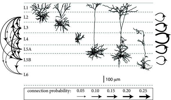
Neurons in different layers of a barrel cortex column have various shapes and form connections with each other with different probabilities (293), indicating that excitatory neurons in the column do not form a homogeneous population; cf. Fig. 12.5. However, if we increase the resolution (i.e., a less ’coarse-grained’ model) to that of a single layer in one barrel cortex column, then it might be possible to consider all excitatory neurons inside one layer as a rather homogeneous population.
12.1.3 Distributed assemblies
The concept of cortical columns suggests that localized populations of neurons can be grouped together into populations, where each population (e.g., the excitatory neurons in layer 4) can be considered as a homogeneous group of neurons with similar intrinsic properties and similar receptive fields. However, the mathematical notion of a population does not require that neurons need to form local groups to qualify as a homogeneous population.
Donald Hebb (210) introduced the notion of neuronal assemblies, i.e., groups of cells which get activated together so as to represent a mental concept such as the preparation of a movement of the right arm toward the left. An assembly can be a group of neurons which are distributed across one or several brain areas. Hence, an assembly is not necessarily a local group of neurons. Despite the fact that neurons belonging to one assembly can be widely distributed, we can think of all neurons belonging to the assembly as a homogeneous population of neurons that is activated whenever the corresponding mental concept is evoked. Importantly, such an assignment of a neuron to a population is not fixed, but can depend on the stimulus. We will return to the concept of distributed assemblies in Chapter 17 when we discuss associative memories and the Hopfield model.