13 Continuity Equation and the Fokker-Planck Approach 13.3 Fokker-Planck equation 13.5 Networks of Nonlinear Integrate-and-Fire Neurons

13.4 Networks of leaky integrate-and-fire neurons

In the previous section, the formalism of membrane potential densities has been applied to a single population driven by spikes arriving at some rate $\nu_{k}$ at the synapse of type $k$ , where $k=1,\dots,K$ . In a population that is coupled to itself, the spikes that drive a given neuron are, at least partially, generated within the same population. For a homogeneous population with self-coupling the feedback is then proportional to the population activity $A(t)$ ; cf. Chapter 12.

We now formulate the interaction between several coupled populations using the Fokker-Planck equation for the membrane potential density (Section 13.4.1) and apply it subsequently to the special cases of a population of excitatory integrate-and-fire neurons interacting with a population of inhibitory ones (Section 13.4.2).

13.4.1 Multiple populations

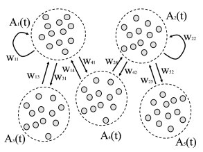
We consider multiple populations $k=1,\dots,K$ . The population with index $k$ contains $N_{k}$ neurons and its activity is denoted by $A_{k}$ . We recall that $N_{k}\,A_{k}(t)\,\Delta t$ is the total number of spikes emitted by population $k$ in a short interval $\Delta t$ .

Let us suppose that population $k$ sends its spikes to another population $n$ . If each neuron in population $n$ receives input from all neurons in $k$ the total spike arrival rate from population $k$ is therefore $\nu_{k}(t)=N_{k}\,A_{k}(t)$ (‘full connectivity’). If each neuron in population $n$ receives connections only from a subset of $C_{nk}$ randomly chosen neurons of population $k$ , then the total spike arrival rate is $\nu_{k}(t)=C_{nk}\,A_{k}(t)$ (’random connectivity’ with a connection probability $p_{nk}=C_{nk}/N_{k}$ from population $k$ to population $n$ ). We assume that all connections from $k$ to $n$ have the same weight $w_{nk}$ .

For each population $n=1,\dots,K$ we write down a Fokker-Planck equation analogous to Eq. (13.16). Neurons are leaky integrate-and-fire neurons. Within a population $n$ , all neurons have the same parameters $\tau_{n}$ , $R_{n}$ , $u_{r}^{n}$ , and in particular the same firing threshold $\vartheta_{n}$ . For population $n$ the Fokker-Planck equation for the evolution of membrane potential densities is then

$\displaystyle\tau_{n}{\partial\over\partial t}p_{n}(u,t)$	$\displaystyle=$	$\displaystyle-{\partial\over\partial u}\left\{\left[-u+R_{n}\,I_{n}^{\rm ext}(% t)+\tau_{n}\sum_{k}C_{nk}A_{k}(t)\,w_{nk}\right]\,p_{n}(u,t)\right\}$	(13.31)
		$\displaystyle+{1\over 2}\,\left[\tau_{n}\sum_{k}C_{nk}A_{k}(t)\,w_{nk}^{2}% \right]\,{\partial^{2}\over\partial u^{2}}p_{n}(u,t)$
		$\displaystyle+\tau_{n}\,A_{n}(t)\,\delta(u-u_{r}^{n})-\tau_{n}\,A_{n}(t)\,% \delta(u-\vartheta_{n})\,.$

The population activity $A_{n}$ is the flux through the threshold (cf. Eq. (13.20)), which gives in our case

A_{n}(t)=-{1\over 2}\,\left[\sum_{k}C_{nk}A_{k}(t)\,w_{nk}^{2}\right]\,\left({% \partial p_{n}(u,t)\over\partial u}\right)_{u=\vartheta_{n}}\,.

(13.32)

Thus populations interact with each other via the variable $A_{k}(t)$ ; cf. Fig. 13.6.

Fig. 13.6: Interacting Populations. A. Five populations interact via their population activities $A_{k}$ . The parameter $w_{nk}$ gives the synaptic weight of a connection from a presynaptic neuron in population $k$ to a postsynaptic neuron in population $n$ . Not all populations are coupled with each other. B. Brunel network: An excitatory population of leaky integrate-and-fire neurons is coupled to itself and to an inhibitory population. Neurons in both populations receive also external input from a third population with population activity $A_{\rm ext}=\nu^{\rm ext}$ described as a homogeneous Poisson process.c

Example: Background input

Sometimes it is useful to focus on a single population, coupled to itself, and replace the input arising from other populations by background input. For example, we may focus on population $n=1$ which is modeled by Eq. (13.31), but use as the inputs $A_{k}$ spikes generated by a homogeneous or inhomogeneous Poisson process with rate $A_{k}=\nu_{k}$ .

Example: Full coupling and random coupling

Full coupling can be retrieved by setting $C_{nk}=N_{k}$ and $w_{nk}=J_{nk}/N_{k}$ . In this case the amount of diffusive noise in population $n$

\sigma_{n}^{2}(t)=\tau_{n}\,\left[\sum_{k}C_{nk}A_{k}(t)\,w_{nk}^{2}\right]\,

(13.33)

decreases with increasing population size $\sigma^{2}_{n}\propto 1/N_{k}$ .

13.4.2 Synchrony, oscillations, and irregularity

In Chapter 12 we have already discussed the stationary state of the population activity in a population coupled to itself. With the methods discussed in Chapter 12 we were, however, unable to study the stability of the stationary state; nor were we able to make any prediction about potential time-dependent solutions.

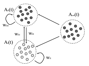
We now give a more complete characterization of a network of leaky integrate-and-fire neurons consisting of two populations: a population of $N_{E}$ excitatory neurons coupled to a population with $N_{I}=N_{E}/4$ inhibitory neurons (79). The structure of the network is shown in Fig. 13.6B. Each neuron (be it excitatory or inhibitory) receives $C_{E}$ connections from the excitatory population each one with weight $w_{EE}=w_{IE}=w_{0}$ ; it also receives $C_{I}=C_{E}/4$ connections from the inhibitory population ( $w_{EI}=w_{II}=-g\,w_{0}$ ) and furthermore $C_{E}$ connections from an external population (weight $w_{EE}$ ) with neurons that fire at a fixed rate $\nu^{\rm ext}$ . Each spike causes, after a delay of $\Delta=1.5ms$ a voltage jump of $w_{0}=0.1$ mV and the threshold is 20mV above resting potential. Note that each neuron receives four times as many excitatory than inhibitory inputs so that the total amount of inhibition balances excitation if inhibition is four times stronger ( $g=4$ ), but the relative strength $g$ is kept as a free parameter. Also note that, in contrast to Chapter 12, the weight here has units of voltage and directly gives the amplitude of the voltage jump: $w_{0}=\Delta u_{E}$ .

Fig. 13.7: Population of pulse-coupled leaky integrate-and-fire neurons (Brunel network). A. Phase diagram of the Brunel network. The population activity can be in a state of asynchronous irregular (AI), synchronous regular (SR) or synchronous irregular (SI) activity. The horizontal axis indicates the relative importance of inhibition ( $g=4$ corresponds to balance between excitation and inhibition). The vertical axis is the amount of external input each neuron receives. Input $I=1$ corresponds to a mean input just sufficient to reach the neuronal firing threshold (in the absence of recurrent input from the network). Stability of the asynchronous irregular firing state (AI) breaks down at the dashed or solid lines and can lead to synchronous regular (SR), or synchronous irregular (SI, either fast or slow) activity, or to a near-quiescent state (Q); redrawn after Brunel (79). B. Typical time course of the population activity $A(t)$ (bottom part of each subgraph, units in kHz) and associated spike patterns (50 randomly chosen neurons are plotted along the vertical axis in the top part of each subgraph, each dot indicates a spike) in different firing regimes. ’SI fast’ refers to fast and regular oscillations, but individual neurons fire irregularly with intervals at random multiples of the oscillation period. Horizontal black bar: 50ms. Simulation of 10 000 excitatory and 2 500 inhibitory neurons with connection probability $p=0.1$ . Each spike causes, after a delay of $\Delta=1.5$ ms a voltage jump of $0.1$ mV; distance from equilibrium potential to threshold is 20mV; absolute refractory period 2ms; membrane time constant $20$ ms. Parameters are top left: $g=3$ , input =2 (SR); top right: $g=6$ , input =4 (SI fast); bottom left: $g=5$ , input =2 (AI) bottom right $g=4.5$ , input =0.9 (SI slow). Adapted from Brunel (79).

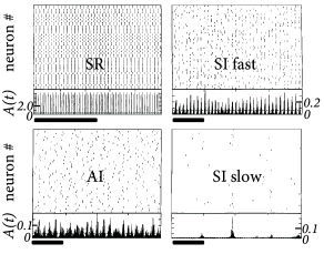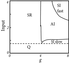
The population can be in a state of asynchronous irregular activity (AI), where neurons in the population fire at different times (’asynchronous’ firing) and the distribution of interspike intervals is fairly broad (’irregular’ firing of individual neurons); cf. Fig. 13.7B. This is the state that corresponds to the considerations of stationary activity in Chapter 12. However, with a slight change of parameters, the same network can also be in a state of fast synchronous regular (SR) oscillations. It is characterized by periodic oscillations of the population activity and a sharply peaked interval distribution of individual neurons. The network can also be in the state of synchronous irregular firing (SI) either with fast (SI fast) or with slow (SI slow) oscillations of the population activity. The oscillatory temporal structure emerges despite the fact that the input has a constant spike arrival rate. It can be traced back to an instability of the asynchronous firing regime toward oscillatory activity.

With the mathematical approach of the Fokker-Planck equations, it is possible to determine the instabilities analytically. The mathematical approach will be presented in Section 13.5.2, but Fig. 13.7A already shows the result. Stability of a stationary state of asynchronous firing is most easily achieved in the regime where inhibition dominates excitation. Since each neuron receives four times as many excitatory as inhibitory inputs, inhibition must be at least four times as strong ( $g>4$ ) as excitation. In order to get non-zero activity despite the strong inhibition, the external input alone must be sufficient to make the neurons fire. ’Input=1’ corresponds to an average external input just sufficient to reach the firing threshold, without additional input from the network.

Consider now the regime of strong inhibition ( $g>4$ ) and strong input, say spikes from the external source arrive at a rate leading to a mean input of amplitude 4. To understand how the network can run into an instability, let us consider the following intuitive argument. Suppose a momentary fluctuation leads to an increase in the total amount of activity in the excitatory population. This causes, after a transmission delay $\Delta$ an increase in inhibition and, after a further delay $\Delta$ a suppression of excitation. If this feedback loop is strong enough, an oscillation with period $4\Delta$ may appear, leading to fast-frequency (’SI fast’) oscillations (79).

If the external input is, on its own, not sufficient to keep the network going (’input $<1$ ’), then a similar small fluctuation may eventually turn the network from a self-activated state into a quiescent state where the only activity is that caused by external input. It then needs another fluctuation (caused by variations of spike arrivals from the external source) to kick it back into a short burst of activity (79). This leads to slow irregular, but synchronous bursts of firing (’SI slow’).

Finally, if inhibition is globally weak compared to excitation ( $g<4$ ), then the population is in a state of high activity where each neuron fires close to its maximal rate (set by the inverse of an absolute refractory period). This high-activity state is unstable compared to fast, but regular oscillations (’SR’). Typically, the population can split up into two or more subgroups, the number of which depends on the transmission delay (79; 181).

Example: Analysis of the Brunel network

All neurons have the same parameters, so that we can assume that they all fire at the same time-dependent firing rate $\nu(t)=A(t)$ . We assume that the network is large $N\gg C_{E}$ , so that it is unlikely that neurons share a large fraction of presynaptic neurons; therefore inputs can be considered as uncorrelated, except for the trivial correlations induced by their common modulation of the firing rate $A(t)$ .

The mean input at time $t$ to a neuron in either the excitatory or the inhibitory population is (in voltage units)

\mu(t)=\tau_{m}\,w_{0}\,C_{E}\,[1-g/4]\,A(t-\Delta)\,+\tau_{m}\,w_{0}\,C_{E}\,% \nu^{\rm ext},

(13.34)

and the input also generates diffusive noise (in voltage units) of strength

\sigma^{2}(t)=\tau_{m}\,{w_{0}^{2}\,C_{E}}[(1+g^{2}/4)A(t-\Delta)+\nu_{\rm ext% }]\,.

(13.35)

The mean and $\sigma^{2}$ are inserted in the Fokker-Planck equation (cf. Eq. 13.31)

$\displaystyle\tau_{m}{\partial\over\partial t}p(u,t)$	$\displaystyle=$	$\displaystyle-{\partial\over\partial u}\left\{\left[-u+\mu(t)\right]\,p(u,t)\right\}$	(13.36)
		$\displaystyle+{1\over 2}\,\sigma^{2}(t)\,{\partial^{2}\over\partial u^{2}}p(u,t)$
		$\displaystyle+\tau_{m}\,A(t)\,\delta(u-u_{r})-\tau_{m}\,A(t)\,\delta(u-% \vartheta)+{\mathcal{O}}(\omega_{k}^{3})\,.$

The main difference to the stationary solution considered in Section 13.3.1 and Chapter 12 is that mean input and noise amplitude are kept time-dependent.

We first solve to find the stationary solution of the Fokker-Planck equation, denoted as $p_{0}(u)$ and activity $A_{0}$ . This step is completely analogous to the calculation in Section 13.3.1.

In order to analyze the stability of the stationary solution, we search for solutions of the form $A(t)=A_{0}+A_{1}\,e^{\lambda t}\,\cos(\omega\,t)$ (for details, see Section 13.5.2). Parameter combinations that lead to a value $\lambda>0$ indicate an instability of the stationary state of asynchronous firing for a network with this set of parameters.

Figure 13.7A indicates that there is a broad regime of stability of the asynchronous irregular firing state (AI). This holds true even if the network is completely deterministic (79) and driven by a constant input $I_{0}$ (i.e., we set $\nu^{\rm ext}=0$ in the noise term, Eq. (13.35), and replace spike arrivals by a constant current $RI_{0}^{\rm ext}=w_{0}C_{E}\,\nu^{\rm ext}$ in Eq. (13.34).

Stability of the stationary state of asynchronous irregular activity is most easily achieved if the network is in the regime where inhibition slightly dominates excitation and external input is sufficient to drive neurons to threshold. This is called the ‘inhibition dominating’ regime. The range of parameters where asynchronous firing is stable can, however, be increased into the range of dominant excitation, if delays are not fixed at $D=1.5$ ms, but drawn from range $0<D<3$ ms. Finite size effects can also be taken into account (79).