16.3 Dynamics of decision making
In this section, we present a mathematical analysis of decision making in models of interacting populations. We start in subsection 16.3.1 with the rate equations for a model with three populations, two excitatory ones which interact with a common inhibitory population. In subsection 16.3.2, the rate model with three populations is reduced to a simplified system described by two differential equations. The fixed points of the two-dimensional dynamical system are analyzed in the phase plane (subsection 16.3.3) for several situations relevant for experiments on decision making. Finally, in subsection 16.3.4 the formalism of competition through shared inhibition is generalized to the case of competing populations.
16.3.1 Model with three populations
In order to analyze the model of Fig. 16.4, we use the rate equations of Chapter 15 and formulate for each of the three interacting populations a differential equation for the input potential. Let
| (16.1) |
denote the population activity of an excitatory population driven by an input potential . Similarly, is the activity of the inhibitory population under the influence of the input potential . Here and are the gain functions of excitatory and inhibitory neurons, respectively. The input potentials evolve according to
| (16.2) | |||||
| (16.3) | |||||
| (16.4) |
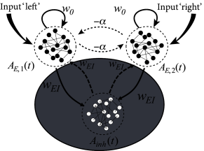
cf. Eqs. (15.3) and (15.1) in Chapter 15. Here denotes the strength of recurrent coupling within each of the excitatory populations and the coupling from the inhibitory to the excitatory population of neurons. Inhibitory neurons are driven by the input from excitatory populations via connections of strength . We assume that inhibitory neurons have no self-coupling, but feed their activity back to both excitatory populations with a negative coupling coefficient, . Note that the two excitatory populations are completely equivalent, i.e. they contain neurons of the same type and the same coupling strength. However, the two populations receive separate inputs, and , respectively. We call an input ‘biased’ (i.e. favoring one of the two options represented by the excitatory populations) if . We emphasize that the only interaction between the two excitatory populations is indirect via the shared inhibitory population.
16.3.2 Effective inhibition
| A | B |
|---|---|
|
 |
The system of three differential equations (16.2) - (16.4) is still relatively complicated. However, from Chapter 4 we know that for a two-dimensional system of equations we can use the powerful mathematical tools of phase plane analysis. This is the main reason why we now reduce the three equations to two.
To do so, we make two assumptions. First, we assume that the membrane time constant of inhibition is shorter than that of excitation, . Formally, we consider the limit of a separation of time scales . Therefore we can treat the dynamics of in Eq. (16.4) as instantaneous, so that the inhibitory potential is always at its fixed point
| (16.5) |
Is this assumption justified? Indeed, inhibitory neurons fire at higher firing rates than excitatory ones and are in this sense ’faster’. However, this observation on its own does not imply that the membrane time constants of excitatory and inhibitory neurons, respectively, would differ by a factor of 10 or more; in fact, they don’t. Nevertheless, a focus on the raw membrane time constant is also too limited in scope, since we should also take into account synaptic processes. Excitatory synapses typically have a NMDA component with time constants in the range of a hundred millisecond or more, whereas inhibitory synapses are fast. We recall from Chapter 15 that the rate equations that we use here are in any case highly simplified and do not fully reflect the potentially much richer dynamics of neuronal populations.
Intuitively, the assumption of a separation of time scale implies that inhibition reacts faster to a change in the input than excitation. In the following we simply assume the separation of time scales between inhibition and excitation, because it enables a significant simplification of the mathematical treatment. Essentially, it means that the variable can be removed from the system of three equations (16.2) - (16.4). Thus we drop Eq. (16.4) and replace in Eqs. (16.2) and (16.3) the input potential by the right-hand side of Eq. (16.5).
The second assumption is not absolutely necessary, but it makes the remaining two equations more transparent. The assumption concerns the shape of the gain function of inhibitory neurons. We require a linear gain function and set
| (16.6) |
with a slope factor . If we insert Eqs. (16.5) and (16.6) into (16.2) and (16.3) we arrive at
| (16.7) | |||||
| (16.8) |
where we have introduced a parameter . Thus, the model of three populations has been replaced by a model with two excitatory populations that interact with an effective inhibitory coupling of strength ; cf. Fig. 16.6A. Even though neurons make either excitatory or inhibitory synapses, but never both (‘Dales law’), the above derivation shows that under appropriate assumptions, there is a mathematically equivalent description where explicit inhibition by inhibitory neurons is replaced by effective inhibition between excitatory neurons. The effective inhibitory coupling allows us to discuss competition between neuronal groups in a transparent manner.
16.3.3 Phase plane analysis
The advantage of the reduced system with two differential equations (16.7) and (16.8) and effective inhibition is that it can be studied using phase plane analysis; cf. Figs. 16.6B and 16.7.
| A | B |
|---|---|
|
 |
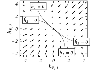
In the absence of stimulation, there exists only a single fixed point , corresponding to a small level of spontaneous activity (Fig. 16.6B).
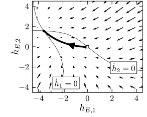
If a stimulus favors the first population, the fixed point moves to an asymmetric position where population 1 exhibits much stronger activity than population 2 (Fig. 16.7A). Note that at the fixed point, . In other words, the effective interaction between the two populations causes a strong inhibitory input potential to population 2. This is a characteristic feature of a competitive network. If one of the populations exhibits a strong activity, it inhibits activity of the others so that only the activity of a single winning population ‘survives’. This principle can also be applied to more than two interacting populations, as we will see in subsection 16.3.4.
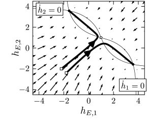
A particularly interesting situation arises with a strong but unbiased stimulus, as we have already seen in the simulations of Fig. 16.5. The phase plane analysis of Fig. 16.7B shows that with a strong unbiased stimulus , three fixed points exist. The symmetric fixed point is a saddle point and therefore unstable. The two other fixed points occur at equivalent positions symmetrically to the left and right of the diagonal. These are the fixed points that enforce a decision ‘left’ or ‘right’.
It depends on the initial conditions or on tiny fluctuations in the noise of the input, whether the system ends up in the left or right fixed point. If, before the onset of the unbiased strong stimulation, the system was at the stable resting point close to , then the dynamics is first attracted toward the saddle point, before it bends over to either the left or right stable fixed point (Fig. 16.7B). Thus, the phase plane analysis of the two-dimensional system correctly reflects the dynamics observed in the simulations of the model with populations of hundreds of spiking neurons (Fig. 16.5B).
16.3.4 Formal winner-take-all networks
| A | B |
|---|---|
|
 |
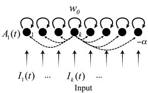
The arguments that were developed above for the case of a binary choice between two options can be generalized to a situation with possible outcomes. Each outcome is represented by one population of excitatory neurons. Analogous to the arguments in Fig. 16.6A, we work with an effective inhibition of strength between the pools of neurons and with a self-interaction of strength within each pool of neurons.
The activity of population is then
| (16.9) |
with input potential
| (16.10) |
where the sum runs over all neurons , except neuron . Note that we assume here a network of interacting populations, but it is common to draw the network as an interaction between formal units. Despite the fact that, in our interpretation, each unit represents a whole population, the units are often called ‘artificial neurons’; cf. Fig. 16.8A. Winner-take-all networks are a standard topic of artificial neural networks (215; 271; 209).
For a suitable choice of coupling parameters and the network implements a competition between artificial neurons, as highlighted in the following example.
Example: Competition
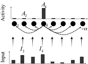
Consider a network of formal neurons described by activities . We work in unit-free variables and set and . Thus, for an input potential the activity is nearly zero while for it is close to one. The input potential, given by Eq. (16.10), contains contributions from external input as well as contributions from recurrent interactions within the network.
Suppose that for all times the external input vanishes, =0 for all . Thus, at time the input potential and the activity are negligible for all units . Therefore the interactions within the network are negligible as well.
At time the input is switched on to a new fixed value which is different for each neuron; cf. Fig. 16.8B. The activity of the neuron which receives the strongest input grows more rapidly than that of the others so that its activity also increases more rapidly. The strong activity of neuron inhibits the development of activity in the other neurons so that, in the end, the neuron with the strongest input wins the competition and its activity is the only one to survive.