Neuron models such as the Spike Response Model with escape noise, formulated in the framework of Generalized Linear Models, can predict spike times of real neurons to a high degree of accuracy; cf. Chapters 9 and 11. We therefore choose the Spike Response Model (SRM) as our candidate for a biologically plausible neuron model. Here we use these neuron models to analyze the macroscopic dynamics in attractor memory networks of spiking neurons.

As discussed in Chapter 9, the membrane potential $u_{i}$ of a neuron $i$ embedded in a large network can be described as

where $\eta(t-t_{i}^{(f)})$ summarizes the refractoriness caused by the spike afterpotential and $h_{i}(t)$ is the (deterministic part of the) input potential

Here $i$ denotes the postsynaptic neuron, $w_{ij}$ is the coupling strength from a presynaptic neuron $j$ to $i$ and $S_{j}(t)=\sum_{f}\delta(t-t_{j}^{(f)})$ is the spike train of neuron $j$.

Statistical fluctuations in the input as well as intrinsic noise sources are both incorporated into an escape rate (or stochastic intensity) $\rho_{i}(t)$ of neuron $i$

which depends on the momentary distance between the (noiseless) membrane potential and the threshold $\vartheta$.

In order to embed memories in the network of SRM neurons we use Eq. (17.27) and proceed as in Section 17.2.6. There are three differences compared to the previous section are: First, while previously $S_{j}$ denoted a binary variable $\pm 1$ in discrete time, we now work with spikes $\delta(t-t_{j}^{(f)})$ in continuous time. Second, in the Hopfield model a neuron can be active in every time step while here spikes must have a minimal distance because of refractoriness. Third, the input potential $h$ is only one of the contributions to the total membrane potential.

Despite these differences the formalism of Section 17.2.6 can be directly applied to the case at hand. Let us define the instantaneous overlap of the spike pattern in the network with pattern $\mu$ as

where $S_{j}(t)=\sum_{f}\delta(t-t_{j}^{(f)})$ is the spike train of neuron $j$. Note that, because of the Dirac $\delta$-function, we need to integrate over $m^{\mu}$ in order to arrive at an observable quantity. Such an integration is automatically performed by each neuron. Indeed, the input potential Eq. (17.34) can be written as

where we have used Eqs. (17.27) and (17.36).

Thus, in a network of $N$ neurons (e.g. $N=100\,000$) which has stored $M$ patterns (e.g., $M=2000$) the input potential is completely characterized by the $M$ overlap variables which reflects an enormous reduction in the complexity of the mathematical problem. Nevertheless, each neuron keeps its identity for two reasons:

(i) Each neuron $i$ is characterized by its ‘private’ set of past firing times $t_{i}^{(f)}$. Therefore each neuron is in a different state of refractoriness and adaptation which manifests itself by the term $\sum_{f}\eta(t-t_{i}^{(f)})$ in the total membrane potential.

(ii) Each neuron has a different functional role during memory retrieval. This role is defined by the sequence $\xi_{i}^{1},\xi_{i}^{2},\dots\xi_{i}^{M}$. For example, if neuron $i$ is part of the active assembly in patterns $\mu=3,\mu=17,\mu=222,\mu=1999$ and should be inactive in the other 1996 patterns, then its functional role is defined by the set of numbers $\xi_{i}^{3}=\xi_{i}^{17}=\xi_{i}^{222}=\xi^{1999}=1$ and $\xi_{i}^{\mu}=0$ otherwise. In a network that stores $M$ different patterns there are $2^{M}$ different functional roles so that it is extremely unlikely that two neurons play the same role. Therefore each of the $N$ neurons in the network is different!

However, during retrieval we can reduce the complexity of the dynamics drastically. Suppose that during the interval $t_{0}<t<t_{0}+T$ all overlaps are negligible, except the overlap with one of the patterns, say pattern $\nu$. Then the input potential in Eq. (17.37) reduces for $t>t_{0}+T$

where we have assumed that $\epsilon(s)=0$ for $s>T$. Therefore, the network with its $N$ different neurons splits up into two homogeneous populations: the first one comprises all neurons with $\xi_{i}^{\nu}=+1$, i.e., those that should be ‘ON’ during retrieval of pattern $\nu$; and the second comprises all neurons with $\xi_{i}^{\nu}=0$, i.e., those that should be ‘OFF’ during retrieval of pattern $\nu$.

In other words, we can apply the mathematical tools of population dynamics that were presented in part III of this book so as to analyze memory retrieval in a network of $N$ different neurons.

Synaptic weights in the Hopfield model can take both positive and negative values. However, in the cortex, all connections originating from the same presynaptic neuron have the same sign, either excitatory or inhibitory. This experimental observation, called Dale’s law, gives rise to a primary classification of neurons as excitatory or inhibitory.

In Chapter 16 we started with models containing separate populations of excitatory and inhibitory neurons, but could show that the model dynamics are, under certain conditions, equivalent to an effective network where the excitatory populations excite themselves but inhibit each other. Thus explicit inhibition was replaced by an effective inhibition. Here we take the inverse approach and transform the effective mutual inhibition of neurons in the Hopfield network into an explicit inhibition via populations of inhibitory neurons.

In order to keep the arguments transparent, let us stick to discrete time and work with random patterns $\xi_{i}^{\mu}\in\{0,1\}$ with mean activity $(\sum_{i}\xi_{i}^{\mu})/N=a$. We take weights $w_{ij}=c^{\prime}\sum_{\mu}(\xi_{i}^{\mu}-b)(\xi_{j}^{\mu}-a)$ and introduce a discrete-time spike variable $\sigma_{i}=0.5(S_{i}+1)$ so that $\sigma_{i}=1$ can be interpreted as a spike and $\sigma_{i}=0$ as the quiescent state. Under the assumption that each pattern $\mu$ has exactly $a\cdot N$ entries with $\xi_{i}^{\mu}=1$, we find that the input potential $h_{i}=\sum_{j}w_{ij}S_{j}$ can be rewritten with the spike variable $\sigma$

In the following we choose $b=0$ and $c^{\prime}=1/4N$. Then the first sum on the right-hand side of Eq. (17.45) describes excitatory and the second one inhibitory interactions.

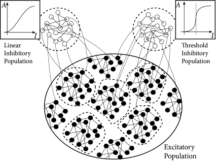
In order to interpret the second term as arising from inhibitory neurons, we make the following assumptions. First, inhibitory neurons have a linear gain function and fire stochastically with probability

where the constant $\gamma$ takes care of the units and $k$ is the index of the inhibitory neuron with $1\leq k\leq N^{\rm inh}$. Second, each inhibitory neuron $k$ receives input from $C$ excitatory neurons. Connections are random and of equal weight $w^{E\to I}=1/C$. Thus, the input potential of neuron $k$ is $h_{k}^{\rm inh}=(1/C)\sum_{j\in\Gamma_{k}}\sigma_{j}$ where $\Gamma_{k}$ is the set of presynaptic neurons. Third, the connection from an inhibitory neuron $k$ back to an excitatory neuron $i$ has weight

Thus, inhibitory weights onto a neuron $i$ which participates in many patterns are stronger than onto one which participates in only a few patterns. Fourth, the number $N^{\rm inh}$ of inhibitory neurons is large. Taken together, the four assumptions give rise to an average inhibitory feedback to each excitatory neuron proportional to $\sum_{j}\sum_{\mu}\xi_{i}^{\mu}\,a\,\sigma_{j}$. In other words, the inhibition caused by the inhibitory population is equivalent to the second term in Eq. (17.45).

Because of our choice $b=0$, patterns are only in weak competition with each other and several patterns can become active at the same time. In order to also limit the total activity of the network, it is useful to add a second pool on inhibitory neurons which turn on whenever the total number of spikes in the network surpasses $a\cdot N$. Note that biological cortical tissue contains many different types of inhibitory interneurons which are thought to play different functional roles.

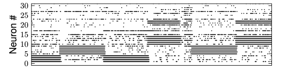
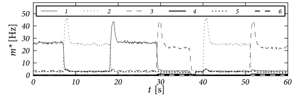
Fig. 17.11 shows that the above argument carry over to the case of integrate-and-fire neurons in continuous time. We emphasize that the network of 8000 excitatory and two groups inhibitory neurons (2000 neurons each) has stored 90 patterns of activity $a\approx 0.1$. Therefore each neuron participates in many patterns (111).

In practice, working memory models with spiking neurons require some parameter tuning. Adding to working models a mechanism of synaptic short-term facilitation (cf. Chapter 3) improves stability of memory retrieval during the delay period (350).