18.3 Bump attractors and spontaneous pattern formation
In this section we study a continuum model with strong recurrent connections such that a spatial activity profile emerges even in cases when the input is homogeneous.
18.3.1 ‘Blobs’ of activity: inhomogeneous states
From a computational point of view bistable systems are of particular interest because they can be used as ‘memory units’. For example a homogeneous population of neurons with all-to-all connections can exhibit a bistable behavior where either all neurons are quiescent or all neurons are firing at their maximum rate. By switching between the inactive and the active state, the neuronal population is able to represent, store, or retrieve one bit of information. The exciting question that arises now is whether a neuronal net with distance-dependent coupling can store more than just a single bit of information, but spatial patterns of activity. Sensory input, e.g., visual stimulation, could switch part of the network to its excited state whereas the unstimulated part would remain in its resting state. Due to bistability this pattern of activity could be preserved even if the stimulation is turned off again and thus provide a neuronal correlate of working memory.
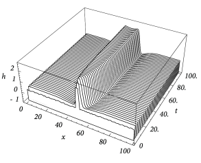
Let us suppose we prepare the network in a state where neurons in one spatial domain are active and all remaining neurons are quiescent. Will the network stay in that configuration? In other words, we are looking for an ‘interesting’ stationary solution of the field equation ( 18.4 ). The borderline where quiescent and active domains of the network meet is obviously most critical to the function of the network as a memory device. To start with the simplest case with a single borderline, we consider a one-dimensional spatial pattern where the activity changes at from the low-activity to the high-activity state. This pattern could be the result of inhomogeneous stimulation in the past, but since we are interested in a memory state we now assume that the external input is simply constant, i.e., . Substitution of into the field equation yields
| (18.29) |
This is a nonlinear integral equation for the unknown function .
We can find a particular solution of Eq. ( 18.29 ) if we replace the output function by a simple step function, e.g.,
| (18.30) |
In this case is either zero or one and we can exploit translation invariance to define for and for without loss of generality. The right-hand side of Eq. ( 18.29 ) does now no longer depend on and we find
| (18.31) |
and in particular
| (18.32) |
with . We have calculated this solution under the assumption that for and for . This assumption imposes a self-consistency condition on the solution, namely that the membrane potential reaches the threshold at . A solution in form of a stationary border between quiescent and active neurons can therefore only be found if
| (18.33) |
If the external stimulation is either smaller or greater than this critical value, then the border will propagate to the right or to the left.
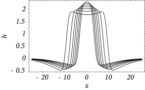
Following the same line of reasoning, we can also look for a localized ‘blob’ of activity. Assuming that for and outside this interval leads to a self-consistency condition of the form
| (18.34) |
with . The mathematical arguments are qualitatively the same, if we replace the step function by a more realistic smooth gain function.
Figure 18.14 shows that solutions in the form of sharply localized excitations exist for a broad range of external stimulations. A simple argument also shows that the width of the blob is stable if ( 17 ) . In this case blobs of activity can be induced without the need of fine tuning the parameters in order to fulfill the self-consistency condition, because the width of the blob will adjust itself until stationarity is reached and Eq. ( 18.34 ) holds; cf. Fig. 18.14 A.
| A | B |
|---|---|
|
|
18.3.2 Sense of Orientation and Head Direction Cells
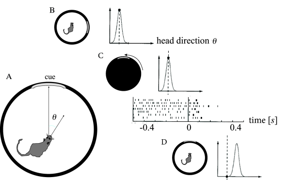
Head direction cells in the rodent entorhinal cortex are thought to be a neural correlate of the internal compass of rodents. A head direction cell responds maximally if the head of the animal points in the direction preferred by this cell ( 508 ) . Different head direction cells have different receptive fields. The preferred direction of head direction cells depends not on absolute north and south, but rather on visual cues. In a laboratory setting, one specific head direction cell will for example always fire when a salient cue card is 60 degree to the left of the body axis, another one when it is 40 degrees to the right (Fig. 18.15 A).
In an experiment during recordings from entorhinal cortex ( 568 ) , a rat was trained to sit still while eating food with its head pointing in the preferred direction of one of the cells in entorhinal cortex. Recordings from this cell show high activity (Fig. 18.15 B). The cell remains active after the light has been switched off indicating that the rat has memorized its momentary orientation. We emphasize that the orientation of the head can be described by a continuous variable. It is therefore this continuous value which needs to be kept in memory!
During the second phase of the experiment, while lights are switched off, the cues are rotated. Finally, in the last phase of the experiment, lights are switched on again. After a few milliseconds, the internal compass aligns with the new position of the cues. The activity of the recorded cell drops (Fig. 18.15 B), because, in the new frame of reference, the head direction is now outside its receptive field ( 568 ) . Two aspects are important from a modeling perspective. First, memory content depends on the external input. Second, the memory must be capable of storing a continuous variable - in contrast to the memory models of Chapter 17 where discrete memory items are stored.
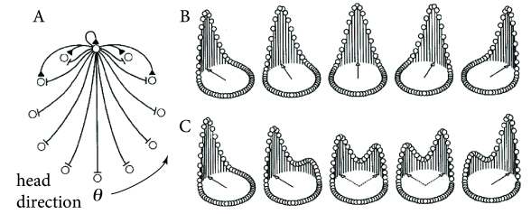
In order to represent the continuous head direction variable, ring models have been used ( 424; 566 ) . The location of a neuron on the ring represents its preferred head direction (Fig. 18.16 ). Cells with similar preferred head direction excite each other whereas cells with opposite preferred head direction inhibit each other. Thus, the ring model has a Mexican-hat connectivity. Parameters are chosen such that the model is in the regime of bump-attractors, so that the present value of presumed head direction is kept in memory, even if stimulation stops.
Example: Activation of Head Direction Cells
Head direction cells rely on visual cues, but also on information arising from the acceleration sensors in the inner ears. One of the intriguing open questions is how the sensory information from the inner ear is transformed into updates of the head direction system ( 424; 566 ) . A second question is how head direction information can be maintained in the absence of further visual or acceleration input. Here we focus on this second question.
Since the activity of head direction cells does not stop when the light is turned off, interactions in a ring model of head direction must be chosen such that activity bumps are stable in the absence of input. Initially, a strong visual cue fixates the bump of activity at one specific location on the ring. If the visual input is switched off, the bump remains at its location so that the past head direction is memorized. When a new input with rotated cues is switched on the activity bump could either rotate towards the new location or disappear at the old and reappear at the new location (Fig. 18.16 ). For large jumps in the input, the latter seems to be more likely in view of the existing experimental data ( 568 ) .