4.6 Separation of time scales and reduction to one dimension

Consider the generic two-dimensional neuron model given by Eqs. (4.4) and (4.5). We measure time in units of $\tau$ and take $R=1$ . Equations (4.4) and (4.5) are then

	$\displaystyle{{\text{d}}u\over{\text{d}}t}$	$\displaystyle=$	$\displaystyle F(u,w)+I$		(4.33)
	$\displaystyle{{\text{d}}w\over{\text{d}}t}$	$\displaystyle=$	$\displaystyle\epsilon\,G(u,w)$		(4.34)

where $\epsilon=\tau/\tau_{w}$ . If $\tau_{w}\gg\tau$ , then $\epsilon\ll 1$ . In this situation the time scale that governs the evolution of $u$ is much faster than that of $w$ . This observation can be exploited for the analysis of the system. The general idea is that of a ‘separation of time scales’; in the mathematical literature the limit of $\epsilon\to 0$ is called ‘singular perturbation’. Oscillatory behavior for small $\epsilon$ is called a ‘relaxation oscillation’.

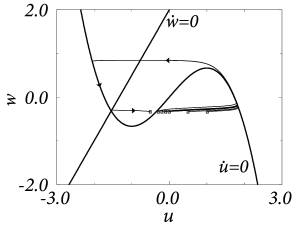
What are the consequences of the large difference of time scales for the phase portrait of the system? Recall that the flow is in direction of $(\dot{u},\dot{w})$ . In the limit of $\epsilon\to 0$ , all arrows in the flow field are therefore horizontal, except those in the neighborhood of the $u$ -nullcline. On the $u$ -nullcline, $\dot{u}=0$ and arrows are vertical as usual. Their length, however, is only of order $\epsilon$ . Intuitively speaking, the horizontal arrows rapidly push the trajectory toward the $u$ -nullcline. Only close to the $u$ -nullcline can directions of movement other than horizontal are possible. Therefore, trajectories slowly follow the $u$ -nullcline, except at the knees of the nullcline where they jump to a different branch.

Excitability can now be discussed with the help of Fig. 4.21. A current pulse shifts the state of the system horizontally away from the stable fixed point. If the current pulse is small, the system returns immediately (i.e., on the fast time scale) to the stable fixed point. If the current pulse is large enough so as to put the system beyond the middle branch of the $u$ -nullcline, then the trajectory is pushed toward the right branch of the $u$ nullcline. The trajectory follows the $u$ -nullcline slowly upward until it jumps back (on the fast time scale) to the left branch of the $u$ -nullcline. The ‘jump’ between the branches of the nullcline corresponds to a rapid voltage change. In terms of neuronal modeling, the jump from the right to the left branch corresponds to the downstroke of the action potential. The middle branch of the $u$ -nullcline (where $\dot{u}>0$ ) acts as a threshold for spike initiation; cf. Fig. 4.22.

If we are not interested in the shape of an action potential, but only in the process of spike initiation, we can exploit the separation of time scales for a further reduction of the two-dimensional system of equations to a single variable. Without input, the neuron is at rest with variables $(u_{\rm rest},w_{\rm rest})^{T}$ . An input current $I(t)$ acts on the voltage dynamics, but has no direct influence on the variable $w$ . Moreover, in the limit of $\epsilon\ll 1$ , the influence of the voltage $u$ on the $w$ -variable via Eq. (4.34) is negligible. Hence, we can set $w=w_{\rm rest}$ and summarize the voltage dynamics of spike initiation by a single equation

\displaystyle{{\text{d}}u\over{\text{d}}t}

\displaystyle=

\displaystyle F(u,w_{\rm rest})+I\,.

(4.35)

Eq. (4.35) is the basis of the nonlinear integrate-and-fire models that we will discuss in Chapter 5.

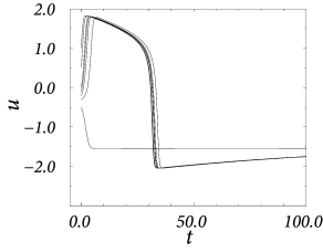
In a two-dimensional neuron model with separation of time scales, the upswing of the spike corresponds to a rapid horizontal movement of the trajectory in the phase plane. The upswing is therefore correctly reproduced by Eq. (4.35). The recovery variable departs from its resting value $w_{\rm rest}$ only during the return of the system to rest, after the voltage has (nearly) reached its maximum (Fig. 4.22A). In the one-dimensional system, the downswing of the action potential is replaced by a simple reset of the voltage variable, as we will see in the next chapter.

Example: Piecewise linear nullclines

Let us study the piecewise linear model shown in Fig. 4.23,

	$\displaystyle{{\text{d}}u\over{\text{d}}t}$	$\displaystyle=$	$\displaystyle f(u)-w+I$		(4.36)
	$\displaystyle{{\text{d}}w\over{\text{d}}t}$	$\displaystyle=$	$\displaystyle\epsilon\,(b\,u-w)$		(4.37)

with $f(u)=a\,u$ for $u<0.5$ , $f(u)=a\,(1-u)$ for $0.5<u<1.5$ and $f(u)=c_{0}+c_{1}\,u$ for $u>1.5$ where $a,c_{1}<0$ are parameters and $c_{0}=-0.5a-1.5c_{1}$ . Furthermore, $b>0$ and $0<\epsilon\ll 1$ .

The rest state is at $u=w=0$ . Suppose that the system is stimulated by a short current pulse that shifts the state of the system horizontally. As long as $u<1$ , we have $f(u)<0$ . According to (4.36), $\dot{u}<0$ and $u$ returns to the rest state. For $u<0.5$ the relaxation to rest is exponential with $u(t)=\exp(a\,t)$ in the limit of $\epsilon\to 0$ . Thus, the return to rest after a small perturbation is governed by the fast time scale.

If the current pulse moves $u$ to a value larger than unity, we have $\dot{u}=f(u)>0$ . Hence the voltage $u$ increases and a pulse is emitted. That is to say, $u=1$ acts as a threshold. Hence, under the assumption of a strict separation of time scales, this neuron model does have a threshold when stimulated with pulse input. The threshold sits on the horizontal axis $w=0$ at the point where $\dot{u}=0$ .

Let us now suppose that the neuron receives a weak and constant background current during our threshold-search experiments. A constant current shifts the $u$ -nullcline vertically upward. Hence the point where $\dot{u}=0$ shifts leftward and therefore the voltage threshold for pulse stimulation sits now at a lower value. Again, we conclude that the threshold value we find depends on the stimulation protocol.