5 Nonlinear Integrate-and-Fire Models 5.2 Exponential Integrate-and-Fire Model 5.4 Summary

5.3 Quadratic Integrate and Fire

A specific instance of a nonlinear integrate-and-fire model is the quadratic model (291; 206),

\tau{{\text{d}}\over{\text{d}}t}u=a_{0}\,(u-u_{\rm rest})\,(u-u_{c})+RI\,,

(5.16)

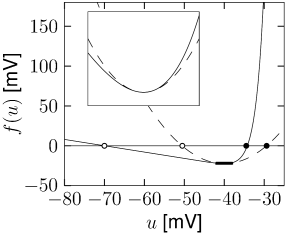
with parameters $a_{0}>0$ and $u_{c}>u_{\rm rest}$ ; cf. Fig. 5.8A. For $I=0$ and initial condition $u<u_{c}$ , the voltage decays to the resting potential $u_{\rm rest}$ . For $u>u_{c}$ it increases so that an action potential is triggered. The parameter $u_{c}$ can therefore be interpreted as the critical voltage for spike initiation by a short current pulse. We will see in the next subsection that the quadratic integrate-and-fire model is closely related to the so-called $\Theta$ -neuron, a canonical type-I neuron model (141; 291).

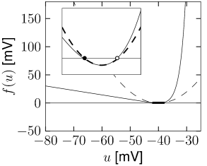
For numerical implementations of the model, the integration of Eq. (5.16) is stopped if the voltage reaches a numerical threshold $\theta_{\rm reset}$ and restarted with a reset value $u_{r}$ as new initial condition (Fig. 5.9B). For a mathematical analysis of the model, however, the standard assumption is $\theta_{\rm reset}\to\infty$ and $u_{r}\to-\infty$ .

We have seen in the previous section that experimental data suggests an exponential, rather than quadratic nonlinearity. However, close to the threshold for repetitive firing, the exponential integrate-and-fire model and the quadratic integrate-and-fire model become very similar (Fig. 5.8B). Therefore the question arises, whether the choice between the two models is a matter of personal preferences only.

For a mathematical analysis, the quadratic integrate-and-fire model is sometimes more handy than the exponential one. However, the fit to experimental data is much better with the exponential than with the quadratic integrate-and-fire model. For a prediction of spike times and voltage of real neurons (cf. Fig. 5.5), it is therefore advisable to work with the exponential rather than the quadratic integrate-and-fire model. Loosely speaking, the quadratic model is too nonlinear in the subthreshold regime and the upswing of a spike is not rapid enough once the voltage is above threshold. The approximation of the exponential integrate-and-fire model by a quadratic one only holds if the mean driving current is close to the rheobase current.

Example: Approximating the exponential integrate-and-fire

Let us suppose that an exponential integrate-and-fire model is driven by a depolarizing current that shifts its effective equilibrium potential $u_{r}^{\rm eff}$ close to the rheobase firing threshold $\vartheta_{rh}$ . The stable fixed points at $u=u_{r}^{\rm eff}$ and the unstable fixed point at $u=\vartheta^{\rm eff}$ corresponding to the effective firing threshold for pulse injection lie now symmetrically around $\vartheta_{rh}$ (Fig. 5.8B). In this region, the shape of the function $f(u)$ is well approximated by a quadratic function (dashed line). In other words, in this regime the exponential and quadratic integrate-and-fire neuron become identical.

If the constant input current is increased further, the stable and unstable fixed point move closer together and finally merge and disappear at the bifurcation point, corresponding to a critical current $I_{c}$ . More generally, any type I neuron model close to the bifurcation point can be approximated by a quadratic integrate-and-fire model - and this is why it is sometimes called the ‘canonical’ type I integrate-and-fire model (141; 140).

Fig. 5.8: Quadratic Integrate-and-Fire Model. A. The quadratic integrate-and-fire model (dashed line), compared to an exponential integrate-and-fire model (solid line). B. The quadratic integrate-and-fire model can be seen as an approximation of an exponential integrate-and-fire model (or any other type I model) depolarized to a state close to repetitive firing. In A and B, the value $f(u)$ and curvature $d^{2}f/du^{2}$ are matched at $u=\vartheta_{rh}$ . Note that the rise in the quadratic model is slower in the super-threshold regime $u>\vartheta_{rh}$ .

Fig. 5.9: Repetitive firing in Nonlinear integrate-and-fire. A Exponential Integrate-and-Fire Model and B Quadratic Integrate-and-Fire Model receiving a constant current sufficient to elicit repetitive firing. Note the comparitively slow upswing of the action potential in the quadratic integrate-and-fire model. Numerical simulation with parameters of equivalent models as illustrated in Fig. 5.8.

5.3.1 Canonical Type I model (*)

In this section, we show that there is a one-to-one relation between the quadratic integrate-and-fire model (5.16) and the canonical type I phase model,

{{\text{d}}\phi\over{\text{d}}t}=[1-\cos\phi]\,+\Delta I\,[1+\cos\phi]\,;

(5.17)

defined in Chapter 4; cf. Section 4.4.1 (141; 140).

Let us denote by $I_{\theta}$ the minimal current necessary for repetitive firing of the quadratic integrate-and-fire neuron. With a suitable shift of the voltage scale and constant current $I=I_{\theta}+\Delta I$ the equation of the quadratic neuron model can then be cast into the form

{{\text{d}}u\over{\text{d}}t}=u^{2}+\Delta I\,.

(5.18)

For $\Delta I>0$ the voltage increases until it reaches the firing threshold $\vartheta\gg 1$ where it is reset to a value $u_{r}\ll-1$ . Note that the firing times are insensitive to the actual values of firing threshold and reset value because the solution of Eq. (5.18) grows faster than exponentially and diverges for finite time (hyperbolic growth). The difference in the firing times for a finite threshold of, say, $\vartheta=10$ and $\vartheta=10\,000$ is thus negligible.

We want to show that the differential equation (5.18) can be transformed into the canonical phase model (5.17) by the transformation

u(t)={\rm tan}\left({\phi(t)\over 2}\right)\,.

(5.19)

To do so, we take the derivative of (5.19) and use the differential equation (5.17) of the generic phase model. With help of the trigonometric relations ${\text{d}}\tan x/{\text{d}}x=1/\cos^{2}(x)$ and $1+\cos x=2\cos^{2}(x/2)$ we find

	$\displaystyle{{\text{d}}u\over{\text{d}}t}$	$\displaystyle=$	$\displaystyle{1\over\cos^{2}(\phi/2)}\,{1\over 2}\,{{\text{d}}\phi\over{\text{% d}}t}$		(5.20)
		$\displaystyle=$	$\displaystyle{\rm tan}^{2}(\phi/2)+\Delta I=u^{2}+\Delta I\,.$		(5.20)

Thus Eq. (5.19) with $\phi(t)$ given by (5.17) is a solution to the differential equation of the quadratic integrate-and-fire neuron. The quadratic integrate-and-fire neuron is therefore (in the limit $\vartheta\to\infty$ and $u_{r}\to-\infty$ ) equivalent to the generic type I neuron (5.17).