6.3 Biophysical Origin of Adaptation
We have introduced, in Section 6.1, formal adaptation variables which evolve according to a linear differential equation (6.2). We now show that the variables can be linked to the biophysics of ion channels and dendrites.
6.3.1 Subthreshold adaptation by a single slow channel
First we focus on one variable at a time and study its subthreshold coupling to the voltage. In other words, the aim is to give a biophysical interpretation of the parameters , , and the variable that show up in the adaptation equation
| (6.15) |
The biophysical components of spike-triggered adaptation (i.e., the interpretation of the reset parameter ) is deferred to Section 6.3.2. Here and in the following we write instead of in order to simplify notation and keep the treatment slightly more general.
As discussed in Chapter 2, neurons contain numerous ion channels (Section 2.3). Rapid activation of the sodium channels, important during the upswing of action potentials, is well approximated (Fig. 5.4) by the exponential nonlinearity in the voltage equation of the AdEx model, Eq. (6.3). We will see now that the subthreshold current is linked to the dynamics of other ion channels with a slower dynamics.
Let us focus on the model of a membrane with a leak current and a single, slow, ion channel, say a potassium channel of the Hodgkin-Huxley type
| (6.16) |
where and are the resistance and reversal potential of the leak current, the membrane time constant, the maximal conductance of the open channel and the gating variable (which appears with arbitrary power ) with dynamics
| (6.17) |
As long as the membrane potential stays below threshold, we can linearize the equations (6.16) and (6.17) around the resting voltage , given by the fixed point condition
| (6.18) |
The resting potential is shifted with respect to the leak reversal potential if the channel is partially open at rest, . We introduce a parameter and expand where is the derivative evaluated at .
The variable then follows the linear equation
| (6.19) |
We emphasize that the time constant of the variable is given by the time constant of the channel at the resting potential. The parameter is proportional to the sensitivity of the channel to a change in the membrane voltage, as measured by the slope at the equilibrium potential .
The adaptation variable is coupled into the voltage equation in the standard form
| (6.20) |
Note that the membrane time constant and the resistance are rescaled by a factor with respect to their values in the passive membrane equation, Eq. ((6.16)). In fact, both are smaller because of partial opening of the channel at rest.
In summary, each channel with nonzero slope at the equilibrium potential gives rise to an effective adaptation variable . Since there are many channels, we can expect many variables . Those with similar time constants can be summed and grouped into a single equation. But if time constants are different by an order of magnitude or more then several adaptation variables are needed, which leads to the model equations (6.1) and (6.2).
6.3.2 Spike-triggered adaptation arising from a biophysical ion-channel
| Type | Fig. | act./inact. | (ms) | (pA) | a (nS) | (pA) | |
|---|---|---|---|---|---|---|---|
| 2.3 | inact. | 20 | -120 | 5.0 | - | - | |
| 2.13 | act. | 61 | 12 | 0.0 | 0.0085 | 0.1 | |
| 2.14 | act. | 33 | 12 | 0.3 | 0.04 | 0.5 | |
| 2.16 | act. | 150 | 12 | 0 | 0.05 | 0.6 | |
| 2.18 | inact. | 8.5 | -48 | 0.8 | - | - | |
| 2.19 | act | 200 | -120 | -0.08 | 0.0041 | -0.48 |
We have seen in Chapter 2 that some ion channels are partially open at the resting potential, while others react only when the membrane potential is well above the firing threshold. We now focus on the second group in order to give a biophysical interpretation of the jump amplitude of a spike-triggered adaptation current.
Let us return to the example of a single ion channel of the Hodgkin and Huxley type such as the potassium current in Eq. (6.16). In contrast to the treatment before, we now study the change in the state of the ion channel induced during the large-amplitude excursion of the voltage trajectory during a spike. During the spike, the target of the gating variable is close to one; but since the time constant is long, the target is not reached during the short time that the voltage stays above the activation threshold. Nevertheless, the ion channel is partially activated by the spike. Unless the neuron is firing at a very large firing rate, each additional spike activate the channel further, always by the same amount , which depends on the duration of the spike and the activation threshold of the current (Table 6.2). The spike-triggered jump in the adapting current is then
| (6.21) |
where has been defined before.
| A |
|
| B |
 |
Again, real neurons with their large quantity of ion channels have many adaptation currents , each with its own time constant , subthreshold coupling and spike-triggered jump . The effective parameter values depend on the properties of the ion channels (Table 6.2).
Example: Calculating the jump of the spike-triggered adaptation current
We consider a gating dynamics
| (6.22) |
with the steplike activation function where mV and ms independent of . Thus, the gating variable approaches a target value of 1 whenever the voltage is above the activation threshold . Since the activation threshold of -30mV is above the firing threshold (typically in the range of -40mV) we can safely state that the neuron activation of the channel can only occur during an action potential. Assuming that, during an action potential the voltage remains for ms above , we can integrate Eq. (6.22) and find that each spike causes an increase where we have exploited that . If we plug in the above numbers, we see that each spike causes an increase of by a value of 0.01. If the duration of the spike were twice as long, the increase would be 0.02. After the spike the gating variable decays with the time constant back to zero. The increase leads to a jump amplitude of the adaptation current given by Eq. (6.21).
6.3.3 Subthreshold adaptation caused by passive dendrites
While in the previous paragraph, we have focused on the role
of ion channels, here we show that a passive
dendrite can also give rise
to a subthreshold coupling of the form of
Eq. (6.15).
We focus on a simple neuron model with two compartments,
representing the soma and the dendrite, superscripts and respectively. The two compartments are both passive with membrane potential , transversal resistance , capacity and resting potential . The two compartments are linked by a longitudinal resistance (see Chapter 3). If current is injected only in the soma, then the two-compartment model with passive dendrites corresponds to
| (6.23) | |||||
| (6.24) |
Such a system of differential equations can be mapped to the form of Eq. (6.15) by considering that the variable represents the current flowing from the dendrite into the soma. In order to keep the treatment transparent, we assume that . In this case the adaptation current is and the two equations above reduce to
| (6.25) | |||||
| (6.26) |
with an effective input resistance , an effective somatic time constant an effective adaptation time constant and a coupling between somatic voltage and adaptation current .
There are three conclusions we should retain from this mapping. First, is always negative, which means that passive dendrites introduce a facilitating subthreshold coupling. Second, facilitation is particularly strong with a small longitudinal resistance. Third, the timescale of the facilitation is smaller than the dendritic time constant - so that, compared to other ‘adaptation’ currents, the dendritic current is a relatively fast one.
In addition to the subthreshold coupling discussed here, dendritic coupling can also lead to a spike-triggered current as we will see in the next example.
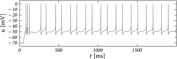
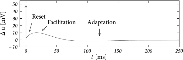
Example: Bursting with a Passive Dendrite and .
Suppose that the action potential can be approximated by a one-millisecond pulse at 0 mV. Then each spike brings an increase in the dendritic membrane potential. In terms of the current , the increase is . Again, the spike-triggered jump is always negative, leading to spike-triggered facilitation. Figure 6.10 shows an example where we combined a dendritic compartment with the linearized effects of the M-current (Table 6.2) to result in regular bursting. The bursting is mediated by the dendritic facilitation which is counterbalanced by the adapting effects of . The firing pattern looks different to the bursting in the AdEx (Fig. 6.4) as there is no alternation between detour and direct resets. Indeed, many different types of bursting are possible (see (238)). This example (especially Fig. 6.10B) suggests that the dynamics of spike-triggered currents on multiple timescales can be understood in terms of their stereotypical effect on the membrane potential - and this insight is the starting point for the Spike Response Model in the next section.