14.2 Recurrent Networks and Interacting Populations
The integral equation (14.5) derived in the previous section can be applied to interacting populations of connected neurons. In Section 14.2.1 we present the mathematical framework of the integral equations so as to describe several populations that interact with each other.
Using the methods discussed in Chapter 12, we can find the activity of a recurrent network in the regime of stationary asynchronous firing (Section 14.2.2). Using the linear response filter, that will be derived in Section 14.3, the stability of the solutions can further be analyzed for different levels of noise and arbitrary delays (Section 14.2.3).
14.2.1 Several populations and networks with self-interaction
In Section 14.1 we discussed a single homogeneous population of neurons. The formalism of integral equations introduced there can readily be adapted to several populations with recurrent interactions within and across populations.
We consider a coupled network of spiking neurons of the renewal type, such as nonlinear (or leaky) integrate-and-fire neurons with escape noise or a Spike Response Model SRM. Neurons within a population have the same set of parameters whereas neurons of different populations can have different parameters. The activity of population is described by Eq. (14.5)
| (14.17) |
where is the input-dependent interval distribution of population . The input to population is
| (14.18) |
Here is the number of neurons in the presynaptic population , is the strength of a synaptic connection of a neuron in population to a neuron in population and the time course of the postsynaptic current into a neuron in population , caused by spike firing of a neuron in population . Conductance-based synapses are treated in the current-based approximation (cf. Section 13.6.3 in Ch. 13). Connections can be excitatory or inhibitory, depending on the choice of . Because the overall strength of the connection is incorporated in , we can, without loss of generality, assume a normalization .
The noise level of each neuron in population is fixed to a value of . The choice of noise is arbitrary. If our aim is to mimic stochastic spike arrivals in randomly connected networks by an escape rate, a suitable choice of escape function has been given in Chapter 9. In practice this implies that noise in the input to a neuron is effectively described and replaced by escape noise in its output.
In the following we assume a fully connected network with interaction strength ; cf. Chapter 12. If the theory is applied to a random network where each neuron in population has a fixed number of presynaptic partners in population , we can use the same theory, except that (i) we use ; and (ii) we increase the noise level in the escape rate function so as to mimic the additional noise caused by stochastic spike arrival; see Section 9.4.
| A | B |
|---|---|

|
 |
14.2.2 Stationary states and fixed points of activity
We are interested in the value of the population activity in the stationary state of asynchronous firing. We recall from Ch. 12 that stationary activity means that the expected value of the population activity is constant whereas in a simulation the actual value always fluctuates (Fig. 14.5). To lighten the notation, we consider a single population with self-interaction and drop the index in the following. The input from other populations is summarized as a constant external input . According the our assumptions, all neurons in the population have the same parameters and can be described by time-dependent renewal theory. The level of noise is indicated by an index .
A stationary state of asynchronous firing requires that the total input is constant (or at least stationary). In Chapter 12, we have seen that the population activity in the state of asynchronous firing is given by the single-neuron firing rate . We thus have
| (14.19) |
Given constant activity of the population and constant external input , the total input to each neuron is constant. From Eq. (14.18) we find the total input to a neuron in population
| (14.20) |
Eq. (14.19) and (14.20) together yield the following equation for the population activity
| (14.21) |
This result agrees with the general result found earlier in Chapter 12 for the stationary state in a network with self-coupling. Solutions can be found graphically (Fig. 14.6) using the same method as in Chapter 12.
The advantage of the integral equation approach is two-fold. First, for the integral-equations we have transparent mathematical tools to analyze the stability of the stationary solution, as shown in Section 14.2.3.
Second, we can write down the gain function and an expression for in a compact form, as will be shown now. Because the input is constant, the state of each neuron depends only on the time since the last spike . We are thus in the situation of stationary renewal theory. Therefore, the survivor function and the interval distribution cannot depend explicitly upon the absolute time, but only on the time difference . Hence we set
| (14.22) | |||||
| (14.23) |
The value of the stationary activity follows now directly from the normalization Eq. (14.8),
| (14.24) |
We use and integrate by parts
| (14.25) |
where the last equality follows from the definition of the mean interspike interval (Chapter 9). Hence
| (14.26) |
The result has an intuitively appealing interpretation: if everything is constant, then averaging over time (for a single neuron) is the same as averaging over a population of identical neurons; cf. the discussion in Chapter 12.
| A | B |
|---|---|
|
 |
Example: Population of SRM neurons with escape noise
Consider a population of SRM neurons with exponential escape noise and membrane potential
| (14.27) |
We assume that the input current is constant so that with . With exponential escape noise, the hazard function (Chapter 9) is and the gain function is given by Eq. (14.26)
| (14.28) |
where indicates the level of noise.
We now set and consider a specific choice of that includes absolute and relative refractoriness
| (14.29) |
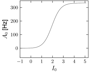
With this choice of it is possible to calculate the gain function in terms of the incomplete gamma function .
| (14.30) |
where (see Exercises). The result is shown in Fig. 14.6A.
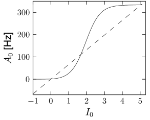
If the population of neurons is coupled to itself with synapses , the stationary value of asynchronous activity can be found graphically by plotting in the same graph and
| (14.31) |
14.2.3 Oscillations and stability of the stationary state (*)
In the previous subsection we have assumed that the network is in a state of asynchronous firing. In this section, we study whether asynchronous firing can indeed be a stable state of a fully connected population of spiking neurons – or whether the connectivity drives the network toward oscillations. For the sake of simplicity, we restrict the analysis to SRM neurons; the same methods can, however, be applied to integrate-and-fire neurons or spiking neurons formulated in the framework of Generalized Linear Models.
For SRM neurons (cf. Chapter 9), the membrane potential is given by
| (14.32) |
where is the effect of the last firing of neuron (i.e., the spike afterpotential) and is the total postsynaptic potential caused by presynaptic firing. If all presynaptic spikes are generated within the homogeneous population under consideration, we have
| (14.33) |
Here is the time course of the postsynaptic potential generated by a spike of neuron at time and is the strength of lateral coupling within the population. The second equality sign follows from the definition of the population activity, i.e., ; cf. Chapter 12. For the sake of simplicity, we have assumed in Eq. (14.33) that there is no external input.
The state of asynchronous firing corresponds to a fixed point of the population activity. We have already seen in the previous subsection as well as in Chapter 12 how the fixed point can be determined either numerically or graphically. To analyze its stability we assume that for the activity is subject to a small perturbation,
| (14.34) |
with . This perturbation in the activity induces a perturbation in the input potential,
| (14.35) |
The perturbation of the potential causes some neurons to fire earlier (when the change in is positive), and others to fire later (whenever the change is negative). The perturbation may therefore build up (, the asynchronous state is unstable) or decay back to zero (, the asynchronous state is stable). At the transition between the region of stability and instability the amplitude of the perturbation remains constant (, marginal stability of the asynchronous state). These transition points, defined by , are determined now.
We start from the population integral equation that has been introduced in Section 14.1. Here is the input-dependent interval distribution, i.e., the probability density of emitting a spike at time given that the last spike occurred at time . The linearized response of the population activity to a small change in the input can, under general smoothness assumptions, always be written in the form
| (14.36) |
where is the linear response filter in the time domain. The Fourier transform is the frequency dependent gain function. The explicit form of the filter will be derived in the framework of the integral equations in Section 14.3.
Instead of thinking of a stimulation by an input current , it is more convenient to work with the input potential , because the neuron model equations have been defined on the level of the potential; cf. Eq. (14.32). We use and in Eq. (14.36) and search for the critical value where the stable solution turns into an unstable one. After cancellation of a common factor the result can be written in the form
| (14.37) |
Here, and are the Fourier transform of the membrane kernel , and the time course of the postsynaptic potential caused by an input spike, respectively. Typically, where is the membrane time constant. If the synaptic input is a short current pulse of unit charge, and are identical, but we would also like to include the case of synaptic input currents with arbitrary time dependence and therefore keep separate symbols for and . The second equality sign defines the real-valued functions and .
Equation (14.37) is thus equivalent to
| (14.38) |
Solutions of Eq. (14.38) yield bifurcation points where the asynchronous firing state looses its stability toward an oscillation with frequency .
We have written Eq. (14.38) as a combination of two requirements, i.e., an amplitude condition and a phase condition . Let us discuss the general structure of the two conditions. First, if for all frequencies , an oscillatory perturbation cannot build up. All oscillations decay and the state of asynchronous firing is stable. We conclude from Eq. (14.37) that by increasing the absolute value of the coupling constant, it is always possible to increase . The amplitude condition can thus be met if the excitatory or inhibitory feedback from other neurons in the population is sufficiently strong. Second, for a bifurcation to occur we need in addition that the phase condition is met. Loosely speaking, the phase condition implies that the feedback from other neurons in the network must arrive just in time to keep the oscillation going. Thus the axonal signal transmission time and the rise time of the postsynaptic potential play a critical role during oscillatory activity (4; 181; 519; 523; 182; 78; 79; 183).
Example: Slow noise and phase diagram of instabilities
Let us apply the above results to leaky integrate-and-fire neurons with slow noise in the parameters. After each spike the neuron is reset to a value which is drawn from a Gaussian distribution with mean and width . After the reset, the membrane potential evolves deterministically according to
| (14.39) |
The next firing occurs if the membrane potential hits the threshold .
We assume that neurons are part of a large population which is in a state of asynchronous firing with activity . In this case, each neuron receives a constant input . For constant input, a neuron which was reset to a value will fire again after a period . Because of the noisy reset with , the interval distribution is approximately a Gaussian centered at . We denote the standard deviation of the interval distribution by . The stationary population activity is simply . The width of the Gaussian interval distribution is linearly related to with a proportionality factor that represents the (inverse of the) slope of the membrane potential at the firing threshold (183).
In order to analyze the stability of the stationary state, we have to specify the time course of the excitatory or inhibitory postsynaptic potential . For the sake of simplicity we choose a delayed alpha function,
| (14.40) |
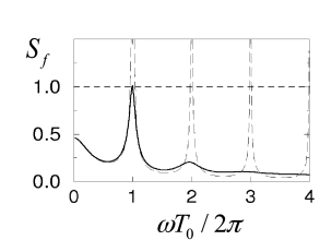
The Fourier transform of has an amplitude and a phase . Note that a change in the delay affects only the phase of the Fourier transform and not the amplitude.
Figure 14.7 shows defined in the second equality sign of Eq. (14.37) as a function of . Since is a necessary condition for a bifurcation, it is apparent that bifurcations can occur only for frequencies with integer where is the typical inter-spike interval. We also see that higher harmonics are only relevant for low levels of noise. At a high noise level, however, the asynchronous state is stable even with respect to perturbations at .
A bifurcation at implies that the period of the perturbation is identical to the firing period of individual neurons. Higher harmonics correspond to instabilities of the asynchronous state toward cluster states (195; 181; 143; 196; 79): each neuron fires with a mean period of , but the population of neurons splits up in several groups that fire alternately so that the overall activity oscillates several times faster. In terms of the terminology introduced in Chapter 13, the network is in the synchronous regular (SR) state of fast oscillations.
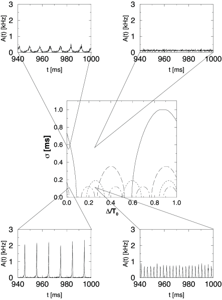
Figure 14.7 illustrates the amplitude condition for the solution of Eq. (14.38). The numerical solutions of the full equation (14.38) for different values of the delay and different levels of the noise are shown in the bifurcation diagram of Fig. 14.8. The insets show simulations that illustrate the behavior of the network at certain combinations of transmission delay and noise level.
Let us consider for example a network with transmission delay ms, corresponding to a -value of in Fig. 14.8. The phase diagram predicts that, at a noise level of ms, the network is in a state of asynchronous firing. The simulation shown in the inset in the upper right-hand corner confirms that the activity fluctuates around a constant value of kHz.
If the noise level of the network is significantly reduced, the system crosses the short-dashed line. This line is the boundary at which the constant activity state becomes unstable with respect to an oscillation with . Accordingly, a network simulation with a noise level of exhibits an oscillation of the population activity with period ms.
Keeping the noise level constant but reducing the transmission delay corresponds to a horizontal move across the phase diagram in Fig. 14.8. At some point, the system crosses the solid line that marks the transition to an instability with frequency . Again, this is confirmed by a simulation shown in the inset in the upper left corner. If we now decrease the noise level, the oscillation becomes even more pronounced (bottom left).
In the limit of low noise, the asynchronous network state is unstable for virtually all values of the delay. The region of the phase diagram in Fig. 14.8 around which looks stable hides instabilities with respect to the higher harmonics and which are not shown. We emphasize that the specific location of the stability borders depends on the form of the postsynaptic response function . The qualitative features of the phase diagram in Fig. 14.8 are generic and hold for all kinds of response kernels.
What happens if the excitatory interaction is replaced by inhibitory coupling? A change in the sign of the interaction corresponds to a phase shift of . For each harmonic, the region along the delay axis where the asynchronous state is unstable for excitatory coupling (cf. Fig. 14.8) becomes stable for inhibition and vice versa. In other words, we simply have to shift the instability tongues for each harmonic frequency horizontally by half the period of the harmonic, i.e. . Apart from that the pattern remains the same.