9 Noisy Output: Escape Rate and Soft Threshold 9.3 Renewal Approximation of the Spike Response Model 9.5 Summary

9.4 From noisy inputs to escape noise

The total input current $I(t)$ which drives a neuron can often be separated into a deterministic component $I^{\rm det}$ , which is known and repeats between one trial and the next; and a stochastic component $\xi$ which is unknown and potentially changes between trials:

I(t)=I^{\rm det}(t)+\xi(t)\,.

(9.25)

In this section we show that the noisy, unknown part in the input can be approximated to a high degree of accuracy by an appropriately chosen escape function.

Example: Adaptive exponential integrate-and-fire model with noisy input

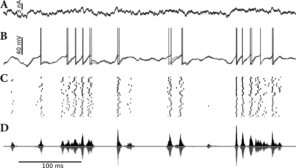
Suppose that the AdEx model which we have encountered in Chapter 6 (see Eqs. (6.3) and (6.4) in Section 6.1) is driven by an input as in Eq. (9.25) containing a rapidly moving deterministic signal $I^{\rm det}(t)$ as well as a white noise component $\xi(t)$ . This model generates spikes with a millisecond precision and a high degree of reliability from one trial to the next (Fig. 9.9). We now approximate the voltage of the AdEx model by a linear model

\displaystyle u(t)=\sum_{f}\eta(t-t_{i}^{(f)})+\int_{0}^{\infty}\kappa(s)\,I^{% \rm det}(t-s)\,{\text{d}}s+u_{\rm rest}\,.

(9.26)

In the subthreshold regime $u<\vartheta-\Delta_{T}$ , the filters $\kappa$ and $\eta$ can be calculated analytically using the methods discussed in Chapter 6. The voltage equation (9.26) is then combined with the exponential escape rate

f(u-\vartheta)={1\over\tau_{0}}\,\exp[\beta\,(u-\vartheta)]\,.

(9.27)

The resulting SRM with escape noise (i.e., a linear model with exponential soft-threshold noise in the output) describes the activity of the AdEx with noisy input (i.e., an exponential neuron model with additive white noise in the input) surprisingly well (Fig. 9.9). In other words, in the presence of an input noise $\xi(t)$ the exponential term in the voltage equation of the AdEx model can be replaced by an exponential escape rate (339).

Fig. 9.9: From input noise to output noise. A. An AdEx model neuron is driven by a fluctuating current containing a deterministic part which is the same during each trial and a stochastic white-noise part. B. Voltage trace of the AdEx model (black) and the SRM with exponential escape rate (gray) during a single trial. The SRM is driven by the determinstic part of the input current. C. Spike times during 20 trials with the same determinstic current for the AdEx model (black) and SRM with exponential escape noise (gray). For the AdEx the stochasticity arises from white noise in the input whereas for the SRM it arises from escape noise in the output. D. Comparison of the PSTH of the AdEx model (black) with that of the SRM (gray). Adapted from Mensi et al. (2011).

9.4.1 Leaky integrate-and-fire model with noisy input

In the subthreshold regime, the leaky integrate-and-fire model with stochastic input (white noise) can be mapped approximately onto an escape noise model with a certain escape rate $f$ (403). In this section, we motivate the mapping and the choice of $f$ .

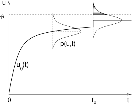
In the absence of a threshold, the membrane potential of an integrate-and-fire model has a Gaussian probability distribution around the noise-free reference trajectory $u_{0}(t)$ . If we take the threshold into account, the probability density at $u=\vartheta$ of the exact solution vanishes, since the threshold acts as an absorbing boundary; see Eq. (8.44). Nevertheless, in a phenomenological model, we can approximate the probability density near $u=\vartheta$ by the ‘free’ distribution (i.e., without the threshold)

{\rm Prob}\big\{u~{}{\rm reaches~{}}\vartheta~{}{\rm in}~{}[t,t+\Delta t]\big% \}\propto\Delta t\,\exp\left\{-{[u_{0}(t)-\vartheta]^{2}\over 2\langle\Delta u% ^{2}(t)\rangle}\right\}\,,

(9.28)

where $u_{0}(t)$ is the noise-free reference trajectory. The idea is illustrated in Fig. 9.10. We note that in a leaky integrate-and-fire model with colored noise in the input (as opposed to white noise) the density at threshold is not zero.

Fig. 9.10: The distribution of the membrane potential around the noise free reference trajectory $u_{0}(t)$ is given by $p(u,t)$ . At $t=t_{0}$ , where the reference trajectory has a discontinuity, the distribution of the membrane potential is shifted instantaneously across the threshold. The probability of firing at $t_{0}$ is given by the shaded surface under the distribution.

We have seen in Eq. (8.13) that the variance $\langle\Delta u^{2}(t)\rangle$ of the free distribution rapidly approaches a constant value $\sigma^{2}/2$ where $\sigma$ scales the strength of the diffusive input. We therefore replace the time dependent variance $2\langle\Delta u(t)^{2}\rangle$ by its stationary value $\sigma^{2}$ . The right-hand side of Eq. (9.28) is then a function of the noise-free reference trajectory only. In order to transform the left-hand side of Eq. (9.28) into an escape rate, we divide both sides by $\Delta t$ . The firing intensity is thus

f(u_{0}-\vartheta)={c_{1}\over\tau_{m}}\,\exp\left\{-{[u_{0}(t)-\vartheta]^{2}% \over\sigma^{2}}\right\}\,.

(9.29)

The factor in front of the exponential has been split into a constant parameter $c_{1}>0$ and the time constant $\tau_{m}$ of the neuron in order to show that the escape rate has units of one over time. Equation (9.29) is the well-known Arrhenius formula for escape across a barrier of height $(\vartheta-u_{0})^{2}$ in the presence of thermal energy $\sigma^{2}$ (529).

Let us now suppose that the neuron receives, at $t=t_{0}$ , an input current pulse which causes a jump of the membrane trajectory by an amount $\Delta u>0$ ; see Fig. (9.10). In this case the Gaussian distribution of membrane potentials is shifted instantaneously across the threshold so that there is a nonzero probability that the neuron fires exactly at $t_{0}$ . To say it differently, the firing intensity $\rho(t)=f[u_{0}(t)-\vartheta]$ has a $\delta$ peak at $t=t_{0}$ . The escape rate of Eq. (9.29), however, cannot reproduce this $\delta$ peak. More generally, whenever the noise free reference trajectory increases with slope $\dot{u}_{0}>0$ , we expect an increase of the instantaneous rate proportional to $\dot{u}_{0}$ , because the tail of the Gaussian distribution drifts across the threshold; cf. Eq. (8.35). In order to take the drift into account, we generalize Eq. (9.29) and study

f(u_{0},\dot{u}_{0})=\left({c_{1}\over\tau_{m}}+{c_{2}\over\sigma}[\dot{u}_{0}% ]_{+}\right)\,\exp\left\{-{[u_{0}(t)-\vartheta]^{2}\over\sigma^{2}}\right\}\,,

(9.30)

where $\dot{u}_{0}={\text{d}}u_{0}/{\text{d}}t$ and $[x]_{+}=x$ for $x>0$ and zero otherwise. We call Eq. (9.30) the Arrhenius&Current model (403).

We emphasize that the right-hand side of Eq. (9.30) depends only on the dimensionless variable

x(t)={u_{0}(t)-\vartheta\over\sigma}\,,

(9.31)

and its derivative $\dot{x}$ . Thus the amplitude of the fluctuations $\sigma$ define a ‘natural’ voltage scale. The only relevant variable is the momentary distance of the noise-free trajectory from the threshold in units of the noise amplitude $\sigma$ . A value of $x=-1$ implies that the membrane potential is one $\sigma$ below threshold. A distance of $u-\vartheta=-10$ mV at high noise (e.g., $\sigma=10$ mV) is as effective in firing a cell as a distance of 1 mV at low noise ( $\sigma=1$ mV).

Example: Comparison of diffusion model and Arrhenius&Current escape rate

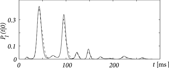
To check the validity of the arguments that led to Eq. (9.30), let us compare the interval distribution generated by the diffusion model with that generated by the Arrhenius&Current escape model. We use the same input potential $u_{0}(t)$ as in Fig. 8.10. We find that the interval distribution for the diffusive white noise model (derived from stochastic spike arrival; see Chapter 8) and that for the Arrhenius&Current escape model are nearly identical; cf. Fig. (9.11). Thus the Arrhenius&Current escape model yields an excellent approximation to the diffusive noise model.

Even though the Arrhenius&Current model has been designed for subthreshold stimuli, it also works remarkably well for superthreshold stimuli. An obvious shortcoming of the escape rate (9.30) is that the instantaneous rate decreases with $u$ for $u>\vartheta$ . The superthreshold behavior can be corrected if we replace the Gaussian $\exp(-x^{2})$ by $2\,\exp(-x^{2})/[1+{\rm erf}(-x)]$ (214). The subthreshold behavior remains unchanged compared to Eq. (9.30) but the superthreshold behavior of the escape rate $f$ becomes linear.

Fig. 9.11: The interval distributions $P_{I}(t|0)$ for diffusive noise (solid line) and Arrhenius&Current escape noise (dashed line) are nearly identical. The input potential is the same as in Fig. 8.10. Taken from (403).

9.4.2 Stochastic resonance

Noise can – under certain circumstances – improve the signal transmission properties of neuronal systems. In most cases there is an optimum for the noise amplitude which has motivated the name stochastic resonance for this rather counterintuitive phenomenon. In this section we discuss stochastic resonance in the context of noisy spiking neurons.

We study the relation between an input $I(t)$ to a neuron and the corresponding output spike train $S(t)=\sum_{f}\delta(t-t^{(f)})$ . In the absence of noise, a subthreshold stimulus $I(t)$ does not generate action potentials so that no information on the temporal structure of the stimulus can be transmitted. In the presence of noise, however, spikes do occur. As we have seen in Eq. (9.30), spike firing is most likely at moments when the normalized distance $|x|=|(u-\vartheta)/\sigma|$ between the membrane potential and the threshold is small. Since the escape rate in Eq. (9.30) depends exponentially on $x^{2}$ , any variation in the membrane potential $u_{0}(t)$ that is generated by the temporal structure of the input is enhanced; cf. Fig. (9.8). On the other hand, for very large noise ( $\sigma\to\infty$ ), we have $x^{2}\to 0$ , and spike firing occurs at a constant rate, irrespective of the temporal structure of the input. We conclude that there is some intermediate noise level where signal transmission is optimal.

The optimal noise level can be found by plotting the signal-to-noise ratio as a function of noise. Even though stochastic resonance does not require periodicity (see, e.g., Collins et al. (101)), it is typically studied with a periodic input signal such as

I^{\rm det}(t)=I_{0}+I_{1}\cos(\Omega\,t)\,.

(9.32)

For $t-\hat{t}\gg\tau_{m}$ , the membrane potential of the noise-free reference trajectory has the form

u_{0}(t)=u_{\infty}+u_{1}\cos(\Omega\,t+\varphi_{1})\,,

(9.33)

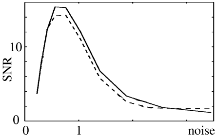
where $u_{1}$ and $\varphi_{1}$ are amplitude and phase of its periodic component. To quantify the signal transmission properties, a long spike train is studied and the signal-to-noise ratio (SNR) is computed. The signal $\mathcal{S}$ is measured as the amplitude of the power spectral density of the spike train evaluated at frequency $\Omega$ , i.e., $\mathcal{S}={{\mathcal{P}}(\Omega)}$ . The noise level $\mathcal{N}$ is usually estimated from the noise power ${\mathcal{P}}_{\rm Poisson}$ of a Poisson process with the same number of spikes as the measured spike train, i.e., $\mathcal{N}={\mathcal{P}}_{\rm Poisson}$ . Figure 9.12 shows the signal-to-noise ratio $\mathcal{S}/\mathcal{N}$ of a periodically stimulated integrate-and-fire neuron as a function of the noise level $\sigma$ . Two models are shown, viz., diffusive noise (solid line) and escape noise with the Arrhenius&Current escape rate (dashed line). The two curves are rather similar and exhibit a peak at

{\sigma^{\rm opt}}\approx{2\over 3}\,(\vartheta-u_{\infty})\,.

(9.34)

Since $\sigma^{2}=2\langle\Delta u^{2}\rangle$ , signal transmission is optimal if the stochastic fluctuations of the membrane potential have an amplitude

2\sqrt{\langle\Delta u^{2}\rangle}\approx\vartheta-u_{\infty}\,.

(9.35)

An optimality condition similar to (9.34) holds over a wide variety of stimulation parameters (406). We will come back to the signal transmission properties of noisy spiking neurons in Chapter 15.

Fig. 9.12: Signal-to-noise ratio (SNR) for the transmission of a periodic signal as a function of the noise level $\sigma/(\vartheta-u_{0})$ . Solid line: Diffusion model. Dashed line: Arrhenius&Current escape model. Taken from (403).

Example: Extracting oscillations

The optimality condition (9.34) can be fulfilled by adapting either the left-hand side or the right-hand side of the equation. Even though it cannot be excluded that a neuron changes its noise level so as to optimize the left-hand side of Eq. (9.34) this does not seem very likely. On the other hand, it is easy to imagine a mechanism that optimizes the right-hand side of Eq. (9.34). For example, an adaptation current could change the value of $\vartheta$ , or synaptic weights could be increased or decreased so that the mean potential $u_{\infty}$ is in the appropriate regime.

We apply the idea of an optimal threshold to a problem of neural coding. More specifically, we study the question whether an integrate-and-fire neuron or a SRM neuron is only sensitive to the total number of spikes that arrive in some time window $T$ , or also to the relative timing of the input spikes. To do so, we compare two different scenarios of stimulation. In the first scenario input spikes arrive with a periodically modulated rate,

\nu^{\rm in}(t)=\nu_{0}+\nu_{1}\,\cos(\Omega\,t)\,

(9.36)

with $0<\nu_{1}<\nu_{0}$ . Thus, even though input spikes arrive stochastically, they have some inherent temporal structure, since they are generated by an inhomogeneous Poisson process. In the second scenario input spikes are generated by a homogeneous (that is, stationary) Poisson process with constant rate $\nu_{0}$ . In a large interval $T\gg\Omega^{-1}$ , however, we expect in both cases a total number of $\nu_{0}\,T$ input spikes.

Stochastic spike arrival leads to a fluctuating membrane potential with variance $\Delta^{2}=\langle\Delta u^{2}\rangle$ . If the membrane potential hits the threshold an output spike is emitted. If stimulus 1 is applied during the time $T$ , the neuron emits a certain number of action potentials, say $n^{(1)}$ . If stimulus 2 is applied it emits $n^{(2)}$ spikes. It is found that the spike count numbers $n^{(1)}$ and $n^{(2)}$ are significantly different if the threshold is in the range

u_{\infty}+\sqrt{\langle\Delta u^{2}\rangle}<\vartheta<u_{\infty}+3\sqrt{% \langle\Delta u^{2}\rangle}\,.

(9.37)

We conclude that a neuron in the subthreshold regime is capable of transforming a temporal code (amplitude $\nu_{1}$ of the variations in the input) into a spike count code (254). Such a transformation plays an important role in the auditory pathway (347; 274; 255).