In this section we develop a density formalism for spike response neurons, similar to the membrane potential density approach for integrate-and-fire neurons that we have discussed in Chapter 13. The main difference is that we replace the membrane potential density $p(u,t)$ by a refractory density $q(r,t)$, to be introduced below.

We study a homogeneous population of neurons with escape noise. The neuron model should be consistent with time-dependent renewal theory. In this case, we can write the membrane potential of a neuron $i$ in general form as

For example, a nonlinear integrate-and-fire model which has fired that last time at $\hat{t}_{i}$ and follows a differential equation $\dot{u}(t^{\prime})=[f(u)+R\,I(t^{\prime})]$ has for $t>\hat{t}_{i}$ a potential $u_{i}(t,\hat{t}_{i})=h(t,\hat{t}_{i})=u_{r}+\int_{\hat{t}_{i}}^{t}\dot{u}(t^{\prime}){\text{d}}t^{\prime}$ and $\eta=0$. A SRM${}_{0}$ neuron has a potential $u_{i}(t,\hat{t})=\eta(t-\hat{t}_{i})+h(t)$ with an arbitrary spike-afterpotential $\eta(t-\hat{t}_{i})$ and an input potential $h$.

The notation in Eq. (14.61) emphasizes the importance of the last firing time $\hat{t}$. We denote the refractory state of a neuron by the variable

i.e., by the time that has passed since the last spike. If we know $r$ and the total input current in the past, we can calculate the membrane potential, $u(t)=\eta(r)+h(t,t-r)$. Given the importance of the refractory variable $r$, we may wonder how many neurons in the population have a refractory state between $r_{0}$ and $r_{0}+\Delta r$. For a large population ($N\to\infty$) the fraction of neurons with a momentary value of $r$ in the interval $[r_{0},r_{0}+\Delta r]$ is given by

where $q(r,t)$ is the refractory density. The aim of this section is to describe the dynamics of a population of SRM neurons by the evolution of $q(r,t)$.

We start from the continuity equation (cf. Ch. 13),

where we have introduced the flux $J_{\rm refr}$ along the axis of the refractory variable $r$. As long as the neuron does not fire, the variable $r=t-\hat{t}$ increases at a speed of ${\text{d}}r/{\text{d}}t=1$. The flux is the density $q$ times the velocity, hence

The continuity equation (14.64) expresses the fact that, as long as a neuron does not fire, its trajectories $r(t)$ can neither start nor end. On the other hand, if a neuron fires, the trajectory stops at the current value of $r$ and ‘reappears’ at $r=0$. In the escape rate formalism, the instantaneous firing rate of a neuron with refractory variable $r$ is given by the hazard

If we multiply the hazard (14.66) with the density $q(r,t)$, we get the loss per unit of time,

The total number of trajectories that disappear at time $t$ due to firing is equal to the population activity, i.e.,

The loss (14.67) has to be added as a ‘sink’ term on the right-hand side of the continuity equation, while the activity $A(t)$ acts as a source at $r=0$. The full dynamics is

This partial differential equation is the analog of the Fokker-Planck equation (13.16) for the membrane potential density of integrate-and-fire neurons. The relation between the two equations will be discussed in Section 14.4.3.

Equation (14.69) can be integrated analytically and rewritten in the form of an integral equation for the population activity. The mathematical details of the integration will be presented below. The final result is

where

is the interval distribution of neurons with escape noise; cf. Eq. (7.28). Thus, neurons that have fired their last spike at time $\hat{t}$ contribute with weight $P_{I}(t|\hat{t})$ to the activity at time $t$. Integral equations of the form (14.70) are the starting point for the formal theory of population activity presented in Section 14.1.

All neurons that have fired together at time $\hat{t}$ form a group that moves along the $r$-axis at constant speed. To solve Eq. (14.69) we turn to a frame of reference that moves along with the group. We replace the variable $r$ by $t-r\equiv\hat{t}$ and define a new density

with $\hat{t}\leq t$. The total derivative of $Q$ with respect to $t$ is

with ${\text{d}}r/{\text{d}}t=1$. We insert Eq. (14.69) on the right-hand side of (14.73) and obtain for $t>\hat{t}$

The partial differential equation (14.69) has thus been transformed into an ordinary differential equation that is solved by

where $Q(\hat{t},t_{0})$ is the initial condition, which is still to be fixed.

From the definition of the refractory density $q(r,t)$ we conclude that $q(0,t)$ is the proportion of neurons at time $t$ that have just fired, i.e., $q(0,t)=A(t)$ or, in terms of the new refractory density, $Q(t,t)=A(t)$. We can thus fix the initial condition in Eq. (14.75) at $t_{0}=\hat{t}$ and find

On the other hand, from (14.68) we have

If we insert (14.76) into (14.77), we find

which is the population equation (14.70) mentioned above. It has been derived from refractory densities in Gerstner and van Hemmen (180) and similarly in the appendix of the papers by Wilson and Cowan (552). If we insert Eq. (14.76) into the normalization condition $1=\int_{-\infty}^{t}Q(\hat{t},t)\,{\text{d}}\hat{t}$ we arrive at

Both the population equation (14.78) and the normalization condition (14.79) play an important role in the general theory outlined in Section 14.1.

For a numerical implementation of population dynamics, it is more convenient to take a step back from the integral equations to the iterative updates that describe the survival $Q(\hat{t},t)$ of the group of neurons that has fired the last time at time $\hat{t}$. In other words, efficient numerical implementation schemes work directly on the level of the density equations (14.74). A simple discretization scheme for numerical implementations has been discussed above in Section 14.1.5.

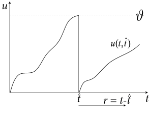
In this section we want to show the formal relation between the dynamics of $p(u,t)$ and the evolution of the refractory densities $q(r,t)$. We focus on a population of nonlinear or leaky integrate-and-fire neurons with escape noise. For a known time-dependent input we can calculate the membrane potential $u(t,\hat{t})$ where the notation with $\hat{t}$ highlights that, in addition to external input, we also need to know the last firing time (and the reset value $u_{r}$) in order to predict the voltage at time $t$. We require that the input is constant or only weakly modulated so that the trajectory is increasing monotonously ($\partial u/\partial t>0$).

To stay concrete, we focus on leaky integrate-and-fire neuron for which the membrane potential is

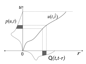
Knowledge of $u(t,\hat{t})$ can be used to define a transformation from voltage to refractory variables: $u\longleftrightarrow r=t-\hat{t}$; cf. Fig. 14.11A. It turns out that the final equations are even simpler if we take $\hat{t}$ instead of $r$ as our new variable. We therefore consider the transformation $u\longrightarrow\hat{t}$.

Before we start, we calculate the derivatives of Eq. (14.80). The derivative with respect to $t$ yields ${\partial u/\partial t}=[-u+R\,I(t)]/\tau_{m}$ as expected for integrate-and-fire neurons. According to our assumption, ${\partial u/\partial t}>0$ or $RI(t)>u$ (for all neurons in the population). The derivative with respect to $\hat{t}$ is

where the function $F$ is defined by Eq. (14.81).

The densities in the variable $\hat{t}$ are denoted as $Q(\hat{t},t)$. From $Q(\hat{t},t)\,{\text{d}}\hat{t}=p(u,t)\,{\text{d}}u$ we have

We now want to show that the differential equation for the density $Q(\hat{t},t)$ that we derived in (14.74),

is equivalent to the partial differential equation for the membrane potential densities. If we insert Eq. (14.82) into Eq. (14.83) we find

For the linear integrate-and-fire neuron we have $\partial F/\partial t=-F/\tau_{m}$. Furthermore, according to our assumption of monotonously increasing trajectories, we have $F\neq 0$. Thus we can divide (14.84) by $F$ and rewrite Eq. (14.84) in the form

where we have used the definition of the hazard via the escape function $\rho(t|\hat{t})=f[u(t,\hat{t})-\vartheta]$ and the definition of the reset potential $u_{r}=\eta_{0}$. If we compare Eq. (14.85) with the Fokker-Planck equation (13.16), we see that the main difference is the treatment of the noise. For noise-free integrate-and-fire neurons (i.e., $\rho(t|\hat{t})=0$ for $u\neq\vartheta$) the equation (13.16) for the membrane potential densities is therefore equivalent to the density equation $\partial Q(\hat{t},t)/\partial t=0$; cf. Eq. (14.83).