7.5 Renewal statistics
Poisson processes do not account for neuronal refractoriness and cannot be used to describe realistic interspike interval distributions. In order to account for neuronal refractoriness in the stochastic description of spike trains, we need to switch from a Poisson process to a renewal process. Renewal process keep a memory of the last event (last firing time ), but not of any earlier events. More precisely, spikes are generated in a renewal process, with a stochastic intensity (or ‘hazard’)
| (7.22) |
which depends on the time since the last spike. One of the simplest example of a renewal system is a Poisson process with absolute refractoriness which we have encountered already in the previous section; see Eq. (7.16).
Renewal processes are a class of stochastic point processes that describe a sequence of events in time (106; 386). Renewal systems in the narrow sense (stationary renewal processes), presuppose stationary input and are defined by the fact that the state of the system, and hence the probability of generating the next event, depends only on the ‘age’ of the system, i.e., the time that has passed since the last event (last spike). The central assumption of renewal theory is that the state does not depend on earlier events (i.e., earlier spikes of the same neuron). The aim of renewal theory is to predict the probability of the next event given the age of the system. In other words, renewal theory allows to calculate the interval distribution
| (7.23) |
i.e., the probability density that the next event occurs at time given that the last event was observed at time .
While for a Poisson process all events occur independently, in a renewal process generation of events (spikes) depends on the previous event, so that events are not independent. However, since the dependence is restricted to the most recent event, intervals between subsequent events are independent. Therefore, an efficient way of generating a spike train of a renewal system is to draw interspike intervals from the distribution .
Example: Light bulb failure as a renewal system
A generic example of a renewal system is a light bulb. The event is the failure of the bulb and its subsequent exchange. Obviously, the state of the system only depends on the age of the current bulb, and not on that of any previous bulb that has already been exchanged. If the usage pattern of the bulbs is stationary (e.g., the bulb is switched on during 10 hours each night) then we have a stationary renewal process. The aim of renewal theory is to calculate the probability of the next failure given the age of the bulb.
7.5.1 Survivor function and hazard
The interval distribution as defined above is a probability density. Thus, integration of over time yields a probability. For example, is the probability that a neuron which has emitted a spike at fires the next action potential between and . Thus
| (7.24) |
is the probability that the neuron stays quiescent between and . is called the survivor function: it gives the probability that the neuron ‘survives’ from to without firing.
The survivor function has an initial value and decreases to zero for . The rate of decay of will be denoted by and is defined by
| (7.25) |
In the language of renewal theory, is called the ‘age-dependent death rate’ or ‘hazard’ (106; 105).
Integration of the differential equation [cf. the first identity in Eq. (7.25)] yields the survivor function
| (7.26) |
According to the definition of the survivor function in Eq. (7.24), the interval distribution is given by
| (7.27) |
which has a nice intuitive interpretation: In order to emit its next spike at , the neuron has to survive the interval without firing and then fire at . The survival probability is and the hazard of firing a spike at time is . Multiplication of the survivor function with the momentary hazard gives the two factors on the right-hand side of Eq. (7.27). Inserting Eq. (7.26) in (7.27), we obtain an explicit expression for the interval distribution in terms of the hazard:
| (7.28) |
On the other hand, given the interval distribution we can derive the hazard from Eq. (7.25). Thus, each of the three quantities , , and is sufficient to describe the statistical properties of a renewal system. Since we focus on stationary renewal systems, the notation can be simplified and Eqs. (7.24)–(7.28) hold with the replacement
| (7.29) | |||||
| (7.30) | |||||
| (7.31) |
Eqs. (7.24) - (7.28) are standard results of renewal theory. The notation that we have chosen in Eqs. (7.24) - (7.28) will turn out to be useful in later chapters and highlights the fact that these quantities are conditional probabilities, probability densities, or rates.
| A | B | C |
|---|---|---|

|

|

|

|

|

|

|

|
 |
Example: From interval distribution to hazard function
Let us suppose that we have found under stationary experimental conditions an interval distribution that can be approximated as
| (7.32) |
with a constant ; cf. Fig. 7.10B. From Eq. (7.25), the hazard is found to be
| (7.33) |
Thus, during an interval after each spike the hazard vanishes. We may interpret as the absolute refractory time of the neuron. For the hazard increases linearly, i.e., the longer the neuron waits the higher its probability of firing. In Chapter 9, the hazard of Eq. (7.33) can be interpreted as the instantaneous rate of a non-leaky integrate-and-fire neuron subject to noise.
7.5.2 Renewal theory and experiments
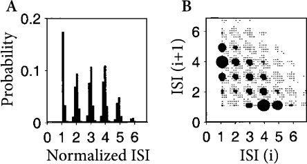
Renewal theory is usually associated with stationary input conditions. The interval distribution can then be estimated experimentally from a single long spike train. The applicability of renewal theory relies on the hypothesis that a memory back to the last spike suffices to describe the spike statistics. In particular, there should be no correlation between one interval and the next. In experiments, the renewal hypothesis, can be tested by measuring the correlation between subsequent intervals. Under some experimental conditions, correlations are small indicating that a description of spiking as a stationary renewal process is a good approximation (192); however, under experimental conditions where neuronal adaptation is strong, intervals are not independent (Fig. 7.11). Given a time series of events with variable intervals , a common measure of memory effects is the serial correlation coefficients
| (7.34) |
Spike-frequency adaptation causes a negative correlation between subsequent intervals (). Long intervals are most likely followed by short ones, and vice versa, so that the assumption of renewal theory does not hold (463; 423; 93).
The notion of stationary input conditions is a mathematical concept that cannot be easily translated into experiments. With intracellular recordings under in vitro conditions, constant input current can be imposed and thus the renewal hypothesis can be tested directly. Under in vivo conditions, the assumption that the input current to a neuron embedded in a large neural system is constant (or has stationary statistics) is questionable; see (392; 393) for a discussion. While the externally controlled stimulus can be made stationary (e.g., a grating drifting at constant speed), the input to an individual neuron is out of control.
Let us suppose that, for a given experiment, we have checked that the renewal hypothesis holds to a reasonable degree of accuracy. From the experimental interval distribution we can then calculate the survivor function and the hazard via Eqs. (7.24) and (7.25). If some additional assumptions regarding the nature of the noise are made, the form of the hazard can be interpreted in terms of neuronal dynamics. In particular, a reduced hazard immediately after a spike is a signature of neuronal refractoriness (192; 52).
Example: Plausible hazard function and interval distributions
Interval distributions and hazard functions have been measured in many experiments. For example, in auditory neurons of the cat driven by stationary stimuli, the hazard function increases, after an absolute refractory time, to a constant level (192). We approximate the time course of the hazard function as
| (7.35) |
with parameters , and ; Fig. 7.10C. In Chapter 9 we will see how the hazard (7.35) can be related to neuronal dynamics. Given the hazard function, we can calculate the survivor function and interval distributions. Application of Eq. (7.26) yields
| (7.36) |
The interval distribution is given by . Interval distribution, survivor function, and hazard are shown in Fig. 7.10C.
We may compare the above hazard function and interval distribution with that of the Poisson neuron with absolute refractoriness. The main difference is that the hazard in Eq. (7.16) jumps from the state of absolute refractoriness to a constant firing rate, whereas in Eq. (7.35) the transition is smooth.
7.5.3 Autocorrelation and noise spectrum of a renewal process (*)
In case of a stationary renewal process, the interval distribution contains all the statistical information so that the autocorrelation function and noise spectrum can be derived. In this section we calculate the noise spectrum of a stationary renewal process. As we have seen above, the noise spectrum of a neuron is directly related to the autocorrelation function of its spike train. Both noise spectrum and autocorrelation function are experimentally accessible.
Let denote the mean firing rate (expected number of spikes per unit time) of the spike train. Thus the probability of finding a spike in a short segment of the spike train is . For large intervals , firing at time is independent from whether or not there was a spike at time . Therefore, the expectation to find a spike at and another spike at approaches for a limiting value . It is convenient to subtract this baseline value and introduce a ‘normalized’ autocorrelation,
| (7.37) |
with . The Fourier transform of Eq. (7.37) yields
| (7.38) |
Thus diverges at ; the divergence is removed by switching to the normalized autocorrelation. In the following we will calculate the noise spectrum for .
| A | B |
|---|---|

|
 |
In the case of a stationary renewal process, the autocorrelation function is closely related to the interval distribution . This relation will now be derived. Let us suppose that we have found a first spike at . To calculate the autocorrelation we need the probability density for a spike at . Let us construct an expression for for . The correlation function for positive will be denoted by or
| (7.39) |
The factor in Eq. (7.39) takes care of the fact that we expect a first spike at with rate . gives the conditional probability density that, given a spike at , we will find another spike at . The spike at can be the first spike after , or the second one, or the th one; see Fig. 7.12. Thus for
| (7.40) | |||||
or
| (7.41) |
as can be seen by inserting Eq. (7.40) on the right-hand side of (7.41); see Fig. 7.13.
Due to the symmetry of , we have for . Finally, for , the autocorrelation has a peak reflecting the trivial autocorrelation of each spike with itself. Hence,
| (7.42) |
In order to solve Eq. (7.41) for we take the Fourier transform of Eq. (7.41) and find
| (7.43) |
Together with the Fourier transform of Eq. (7.42), , we obtain
| (7.44) |
For , the Fourier integral over the right-hand side of Eq. (7.40) diverges, since . If we add the diverging term from Eq. (7.38), we arrive at
| (7.45) |
This is a standard result of stationary renewal theory (105) which has been repeatedly applied to neuronal spike trains (137; 36).
Example: Stationary Poisson process
In Section 7.2.1 and Section 7.5 we have already discussed the Poisson neuron from the perspective of mean firing rate and renewal theory, respectively. The autocorrelation of a Poisson process is
| (7.46) |
We want to show that Eq. (7.46) follows from Eq. (7.40).
Since the interval distribution of a Poisson process is exponential [cf. Eq. (7.16) with ], we can evaluate the integrals on the right-hand side of Eq. (7.40) in a straightforward manner. The result is
| (7.47) |
Hence, with Eq. (7.42), we obtain the autocorrelation function (7.46) of a homogeneous Poisson process. The Fourier transform of Eq. (7.46) yields a flat spectrum with a peak at zero:
| (7.48) |
The result could have also been obtained by evaluating Eq. (7.45).
Example: Poisson process with absolute refractoriness
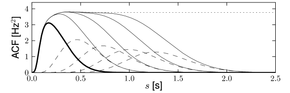
We return to the Poisson process with absolute refractoriness defined in Eq. (7.16). Apart from an absolute refractory time , the neuron fires with rate . For , Eq. (7.45) yields the noise spectrum
| (7.49) |
cf. Fig. (7.12)B. In contrast to the stationary Poisson process Eq. (7.46), the noise spectrum of a neuron with absolute refractoriness is no longer flat. In particular, for , the noise spectrum is decreased by a factor . Eq. (7.49) and generalizations thereof have been used to fit the power spectrum of, e.g., auditory neurons (137) and MT neurons (36).
Can we understand the decrease in the noise spectrum for ? The mean interval of a Poisson neuron with absolute refractoriness is . Hence the mean firing rate is
| (7.50) |
For we retrieve the stationary Poisson process Eq. (7.3) with . For finite the firing is more regular than that of a Poisson process with the same mean rate . We note that for finite , the mean firing rate remains bounded even if . The neuron fires then regularly with period . Because the spike train of a neuron with refractoriness is more regular than that of a Poisson neuron with the same mean rate, the spike count over a long interval, and hence the spectrum for , is less noisy. This means that Poisson neurons with absolute refractoriness can transmit slow signals more reliably than a simple Poisson process.
7.5.4 Input dependent renewal theory (*)
It is possible to use the renewal concept in a broader sense and define a renewal process as a system where the state at time (and hence the probability of generating an event at ), depends both on the time that has passed since the last event (i.e., the firing time ) and the input , , that the system received since the last event. Input-dependent renewal systems are also called modulated renewal processes (425), non-stationary renewal systems (182; 183), or inhomogeneous Markov interval processes (251). The aim of a theory of input-dependent renewal systems is to predict the probability density
| (7.51) |
of the next event to occur at time , given the timing of the last event and the input for ; see Fig. 7.14. The relation between hazard, survivor function, and interval distribution for the input-dependent case is the same as the one given in Equations (7.25) – (7.28). The generalization to a time-dependent renewal theory will be useful later on in Chapter 9.
The lower index of is intended to remind the reader that the probability density depends on the time course of the input for . Since is conditioned on the spike at , it can be called a spike-triggered spike density. We interpret as the distribution of interspike intervals in the presence of an input current or as the input-dependent interval distribution. For stationary input, reduces to .
| A | B |
|---|---|
 |
|