3 Dendrites and Synapses 3.1 Synapses 3.3 Spatial Structure: Axons

3.2 Spatial Structure: The Dendritic Tree

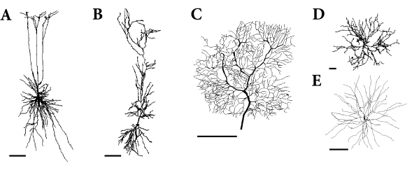
Fig. 3.4: Reconstructed morphology of various types of neurons. A. Pyramidal neuron from a deep cortical layer(103). B. Pyramidal neuron from the CA1 of the hippocampus (193). C. Purkinje cell from the cerebellum (420). D. Motoneuron from the spinal cord (110). E. Stellate neuron from the neocortex (325). Reconstructed morphologies can be downloaded from http://NeuroMorpho.Org. Scale bars represents 100 $\mu m$ .

Neurons in the cortex and other areas of the brain often exhibit highly developed dendritic trees that may extend over several hundred microns (Fig. 3.4). Synaptic input to a neuron is mostly located on its dendritic tree. Disregarding NMDA- or Calcium-based electrogenic ‘spikes’, action potentials are generated at the soma near the axon hillock. Up to now we have discussed point neurons only, i.e., neurons without any spatial structure. What are the consequences of the spatial separation of input and output?

The electrical properties of point neurons have been described as a capacitor that is charged by synaptic currents and other transversal ion currents across the membrane. A non-uniform distribution of the membrane potential on the dendritic tree and the soma induces additional longitudinal current along the dendrite. We are now going to derive the cable equation that describes the membrane potential along a dendrite as a function of time and space. In Section 3.4 we will see how geometric and electrophysiological properties can be integrated in a comprehensive biophysical model.

3.2.1 Derivation of the Cable Equation

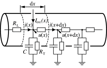
Consider a piece of dendrite decomposed into short cylindric segments of length ${\text{d}}x$ each. The schematic drawing in Fig. 3.5 shows the corresponding circuit diagram. Using Kirchhoff’s laws we find equations that relate the voltage $u(x)$ across the membrane at location $x$ with longitudinal and transversal currents. First, a longitudinal current $i(x)$ passing through the dendrite causes a voltage drop across the longitudinal resistor $R_{\text{L}}$ according to Ohm’s law,

u(t,x+{\text{d}}x)-u(t,x)=R_{\text{L}}\,i(t,x)\,,

(3.9)

where $u(t,x+{\text{d}}x)$ is the membrane potential at the neighbouring point $x+{\text{d}}x$ . Second, the transversal current that passes through the RC-circuit is given by $C\,\partial u(t,x)/\partial t+\sum_{ion}I_{ion}$ where the sum runs over all ion channel types present in the dendrite. Kirchhoff’s law regarding the conservation of current at each node leads to

i(t,x+{\text{d}}x)-i(t,x)=C\,\frac{\partial}{\partial t}\,u(t,x)+\sum_{ion}I_{% ion}-I_{\text{ext}}(t,x)\,.

(3.10)

The values of the longitudinal resistance $R_{\text{L}}$ , the capacity $C$ , the ionic currents as well as the externally applied current can be expressed in terms of specific quantities per unit length $r_{\text{L}}$ , $c$ , $i_{ion}$ and $i_{\text{ext}}$ , respectively, viz.

R_{\text{L}}=r_{\text{L}}\,{\text{d}}x\,,\quad C=c\,{\text{d}}x\,,\quad I_{% \text{ext}}(t,x)=i_{\text{ext}}(t,x)\,{\text{d}}x\quad I_{ion}(t,x)=i_{ion}(t,% x)\,{\text{d}}x\,.

(3.11)

These scaling relations express the fact that the longitudinal resistance and the capacity increases with the length of the cylinder. Similarly, the total amount of transversal current increases with the length ${\text{d}}x$ simply because the surface through which the current can pass is increasing. Substituting these expressions in Eqs. (3.9) and (3.10), dividing by ${\text{d}}x$ , and taking the limit ${\text{d}}x\to 0$ leads to

	$\displaystyle\frac{\partial}{\partial x}\,u(t,x)$	$\displaystyle=r_{\text{L}}\,i(t,x)$		(3.12a)
	$\displaystyle\frac{\partial}{\partial x}\,i(t,x)$	$\displaystyle=c\,\frac{\partial}{\partial t}\,u(t,x)+\sum_{ion}i_{ion}(t,x)-i_% {\text{ext}}(t,x)\,.$		(3.12b)

Taking the derivative of equation (3.12a) with respect to $x$ and substituting the result into (3.12b) yields

\frac{\partial^{2}}{\partial x^{2}}\,u(t,x)=c\,r_{\text{L}}\,\frac{\partial}{% \partial t}\,u(t,x)+r_{\text{L}}\sum_{ion}i_{ion}(t,x)-r_{\text{L}}\,i_{\text{% ext}}(t,x).

(3.13)

Eq. (3.13) is called the general cable equation.

Fig. 3.5: Part of a dendrite and the corresponding circuit diagram. Longitudinal and transversal resistors are denoted by $R_{\text{L}}$ and $R_{\text{T}}$ , respectively. The electrical capacity of each small piece of dendrite is symbolized by capacitors $C$ .

Example: Cable equation for passive dendrite

The ionic currents $\sum_{ion}i_{ion}(t,x)$ in Eq. (3.13) can in principle comprise many different types of ion channel, as discussed in Chapter 2.3. For simplicity, the dendrite is sometimes considered as passive. This means that the current density follows Ohms law $\sum_{ion}i_{ion}(t,x)=g_{l}\,(u-E_{l})$ where $g_{l}=1/r_{\text{T}}$ is the leak conductance per unit length and $E_{l}$ is the leak reversal potential.

We introduce the characteristic length scale $\lambda^{2}=r_{\text{T}}/r_{\text{L}}$ (“electrotonic length scale”) and the membrane time constant $\tau=r_{\text{T}}\,c$ . If we multiply Eq. (3.13) by $\lambda^{2}$ we get

\lambda^{2}\,\frac{\partial^{2}}{\partial x^{2}}\,u(t,x)=\tau\,\frac{\partial}% {\partial t}\,u(t,x)+[u(t,x)-E_{l}]-r_{\text{T}}\,i_{\text{ext}}(t,x).

(3.14)

After a transformation to unit-free coordinates,

x\to\hat{x}=x/\lambda\,,\quad t\to\hat{t}=t/\tau\,,

(3.15)

and a rescaling of the current and voltage variables,

i\to\hat{i}=\sqrt{r_{\text{T}}\,r_{\text{L}}}\;i\,,\quad i_{\text{ext}}\to\hat% {i}_{\text{ext}}=r_{\text{T}}\,i_{\text{ext}}\,,\quad u\to\hat{u}=u-E_{l},

(3.16)

we obtain the cable equation (where we have dropped the hats)

\frac{\partial}{\partial t}\,u(t,x)=\frac{\partial^{2}}{\partial x^{2}}\,u(t,x% )-u(t,x)+i_{\text{ext}}(t,x),

(3.17)

in an elegant unit-free form.

The cable equation can be easily interpreted. The change in time of the voltage at location $x$ is determined by three different contributions. The first term on the right-hand side of Eq. (3.17) is a diffusion term that is positive if the voltage is a convex function of $x$ . The voltage at $x$ thus tends to increase, if the values of $u$ are higher in a neighborhood of $x$ than at $x$ itself. The second term on the right-hand side of Eq. (3.17) is a simple decay term that causes the voltage to decay exponentially towards zero. The third term, finally, is a source term that acts as an inhomogeneity in the otherwise autonomous differential equation. This source can be due to an externally applied current or to synaptic input arriving at location $x$

Example: Stationary solutions of the cable equation

In order to get an intuitive understanding of the behavior of the cable equation of a passive dendrite we look for stationary solutions of Eq. (3.17), i.e., for solutions with $\partial u(t,x)/\partial t=0$ . In that case, the partial differential equation reduces to an ordinary differential equation in $x$ , viz.

\frac{\partial^{2}}{\partial x^{2}}\,u(t,x)-u(t,x)=-i_{\text{ext}}(t,x)\,.

(3.18)

The general solution to the homogenous equation with $i_{\text{ext}}(t,x)\equiv 0$ is

u(t,x)=c_{1}\,\sinh(x)+c_{2}\,\cosh(x)\,,

(3.19)

as can easily be checked by taking the second derivative with respect to $x$ . Here, $c_{1}$ and $c_{2}$ are constants that are determined by the boundary conditions.

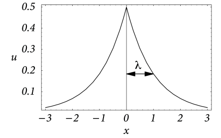
Solutions for non-vanishing input current can be found by standard techniques. For a stationary input current $i_{\text{ext}}(t,x)=\delta(x)$ localized at $x=0$ and boundary conditions $u(\pm\infty)=0$ we find

u(t,x)=\frac{1}{2}\,{\text{e}}^{-\left|x\right|}\,,

(3.20)

cf. Fig. 3.6. This solution is given in units of the intrinsic length scale $\lambda=(r_{\text{T}}/r_{\text{L}})^{1/2}$ . If we re-substitute the physical units, we see that $\lambda$ is the length over which the stationary membrane potential drops by a factor $1/{\text{e}}$ . In the literature $\lambda$ is referred to as the electrotonic length scale (414). Typical values for the specific resistance of the intracellular medium and the cell membrane are $100\,\Omega\,\text{cm}$ and $30\,\text{k}\Omega\,\text{cm}^{2}$ , respectively. In a dendrite with radius $\rho=1\,\mu$ m this amounts to a transversal and a longitudinal resistance of $r_{\text{L}}=100\,\Omega\,\text{cm}/(\pi\rho^{2})=3\cdot 10^{5}\,\Omega\,\mu% \text{m}^{-1}$ and $r_{\text{T}}=30\,\text{k}\Omega\,\text{cm}^{2}/(2\pi\rho)=5\cdot 10^{11}\,% \Omega\,\mu\text{m}$ . The corresponding electrotonic length scale is $\lambda=1.2\,\text{mm}$ . Note that the electrotonic length can be significantly smaller if the transversal conductivity is increased, e.g., due to open ion channels.

For arbitrary stationary input current $i_{\text{ext}}(x)$ the solution of Eq. (3.17) can be found by a superposition of translated fundamental solutions (3.20), viz.,

u(t,x)=\int\!\!{\text{d}}x^{\prime}\;\frac{1}{2}\,{\text{e}}^{-\left|x-x^{% \prime}\right|}\,i_{\text{ext}}(x^{\prime})\,.

(3.21)

This is an example of the Green’s function approach applied here to the stationary case. The general time-dependent case will be treated in the next section.

Fig. 3.6: Stationary solution of the cable equation with a constant current of unit strength being injected at $x=0$ , i.e., $i_{\text{ext}}(t,x)=\delta(x)$ . The electrotonic length scale $\lambda$ is the distance over which the membrane potential drops to $1/{\text{e}}$ of its initial value.

3.2.2 Green’s Function of the passive Cable

In the following we will concentrate on the equation for the voltage and start our analysis by a discussion of the Green’s function for a cable extending to infinity in both directions. The Green’s function is defined as the solution of a linear equation such as Eq. (3.17) with a Dirac $\delta$ -pulse as its input. It can be seen as an elementary solution of the differential equation because – due to linearity – the solution for any given input can be constructed as a superposition of these Green’s functions.

Suppose a short current pulse $i_{\text{ext}}(t,x)$ is injected at time $t=0$ at location $x=0$ . As we will show below, the time course of the voltage at an arbitrary position $x$ is given by

u(t,x)=\frac{\Theta(t)}{\sqrt{4\pi\,t}}\,\exp\left[-t-\frac{x^{2}}{4\,t}\right% ]\equiv G_{\infty}(t,x)\,,

(3.22)

where $G_{\infty}(t,x)$ is the Green’s function. Knowing the Green’s function, the general solution for an infinitely long cable is given by

u(t,x)=\int_{-\infty}^{t}\!\!{\text{d}}t^{\prime}\int_{-\infty}^{\infty}\!\!{% \text{d}}x^{\prime}\;G_{\infty}(t-t^{\prime},x-x^{\prime})\,i_{\text{ext}}(t^{% \prime},x^{\prime})\,.

(3.23)

The Green’s function is therefore a particularly elegant and useful mathematical tool: once you have solved the linear cable equation for a single short current pulse, you can write down the full solution to arbitrary input as an integral over (hypothetical) pulse-inputs at all places and all times.

Checking the Green’s property*

We can check the validity of Eq. (3.22) by substituting $G_{\infty}(t,x)$ into Eq. (3.17). After a short calculation we find

\left[\frac{\partial}{\partial t}-\frac{\partial^{2}}{\partial x^{2}}+1\right]% \,G_{\infty}(t,x)=\frac{1}{\sqrt{4\pi\,t}}\,\exp\left(-t-\frac{x^{2}}{4t}% \right)\,\delta(t)\,,

(3.24)

where we have used $\partial\Theta(t)/\partial t=\delta(t)$ . As long as $t\neq 0$ the right-hand side of Eq. (3.24) vanishes, as required by Eq. (3.28). For $t\to 0$ we find

\lim_{t\to 0}\frac{1}{\sqrt{4\pi\,t}}\,\exp\left(-t-\frac{x^{2}}{4t}\right)=% \delta(x)\,,

(3.25)

which proves that the right-hand side of Eq. (3.24) is indeed equivalent to the right-hand side of Eq. (3.28).

Having established that

\left[\frac{\partial}{\partial t}-\frac{\partial^{2}}{\partial x^{2}}+1\right]% \,G_{\infty}(t,x)=\delta(x)\,\delta(t)\,,

(3.26)

we can readily show that Eq. (3.23) is the general solution of the cable equation for arbitrary input currents $i_{\text{ext}}(t_{0},x_{0})$ . We substitute Eq. (3.23) into the cable equation, exchange the order of integration and differentiation, and find

\left[\frac{\partial}{\partial t}-\frac{\partial^{2}}{\partial x^{2}}+1\right]% \,u(t,x)=\\ =\int_{-\infty}^{t}\!\!{\text{d}}t^{\prime}\int_{-\infty}^{\infty}\!\!{\text{d% }}x^{\prime}\;\left[\frac{\partial}{\partial t}-\frac{\partial^{2}}{\partial x% ^{2}}+1\right]\,G_{\infty}(t-t^{\prime},x-x^{\prime})\,i_{\text{ext}}(t^{% \prime},x^{\prime})=\\ =\int_{-\infty}^{t}\!\!{\text{d}}t^{\prime}\int_{-\infty}^{\infty}\!\!{\text{d% }}x^{\prime}\;\delta(x-x^{\prime})\,\delta(t-t^{\prime})\,i_{\text{ext}}(t^{% \prime},x^{\prime})=i_{\text{ext}}(t,x)\,.

(3.27)

Derivation of the Green’s function (*)

Previously, we have just ‘guessed’ the Green’s function and then shown that it is indeed a solution of the cable equation. However, it is also possible to derive the Green’s function step by step. In order to find the Green’s function for the cable equation we thus have to solve Eq. (3.17) with $i_{\text{ext}}(t,x)$ replaced by a $\delta$ impulse at $x=0$ and $t=0$ .

\frac{\partial}{\partial t}\,u(t,x)-\frac{\partial^{2}}{\partial x^{2}}\,u(t,x% )+u(t,x)=\delta(t)\,\delta(x)\,.

(3.28)

Fourier transformation with respect to the spatial variable yields

\frac{\partial}{\partial t}\,\tilde{u}(t,k)+k^{2}\,\tilde{u}(t,k)+\tilde{u}(t,k)=\delta(t)/\sqrt{2\pi}\,.

(3.29)

This is an ordinary differential equation in $t$ and has a solution of the form

\tilde{u}(t,k)=\exp\left[-\left(1+k^{2}\right)\,t\right]/\sqrt{2\pi}\,\Theta(t),

(3.30)

with $\Theta(t)$ denoting the Heaviside function. After an inverse Fourier transform we obtain the desired Green’s function $G_{\infty}(t,x)$ ,

u(t,x)=\frac{\Theta(t)}{\sqrt{4\pi\,t}}\,\exp\left[-t-\frac{x^{2}}{4\,t}\right% ]\equiv G_{\infty}(t,x)\,.

(3.31)

Example: Finite cable

Real cables do not extend from $-\infty$ to $+\infty$ and we have to take extra care to correctly include boundary conditions at the ends. We consider a finite cable extending from $x=0$ to $x=L$ with sealed ends, i.e., $i(t,x=0)=i(t,x=L)=0$ or, equivalently, $\frac{\partial}{\partial x}u(t,x=0)=\frac{\partial}{\partial x}u(t,x=L)=0$ .

The Green’s function $G_{0,L}$ for a cable with sealed ends can be constructed from $G_{\infty}$ by applying a trick from electro-statics called “mirror charges” (240). Similar techniques can also be applied to treat branching points in a dendritic tree (5). The cable equation is linear and, therefore, a superposition of two solutions is also a solution. Consider a $\delta$ current pulse at time $t_{0}$ and position $x_{0}$ somewhere along the cable. The boundary condition $\frac{\partial}{\partial x}u(t,x=0)=0$ can be satisfied if we add a second, virtual current pulse at a position $x=-x_{0}$ outside the interval $[0,L]$ . Adding a current pulse outside the interval $[0,L]$ comes for free since the result is still a solution of the cable equation on that interval. Similarly, we can fulfill the boundary condition at $x=L$ by adding a mirror pulse at $x=2\,L-x_{0}$ . In order to account for both boundary conditions simultaneously, we have to compensate for the mirror pulse at $-x_{0}$ by adding another mirror pulse at $2\,L+x_{0}$ and for the mirror pulse at $x=2\,L-x_{0}$ by adding a fourth pulse at $-2\,L+x_{0}$ and so forth. Altogether we have

G_{0,L}(t_{0},x_{0};t,x)=\inner@par\sum_{n=-\infty}^{\infty}G_{\infty}(t-t_{0}% ,x-2\,n\,L-x_{0})+G_{\infty}(t-t_{0},x-2\,n\,L+x_{0})\,.

(3.32)

We emphasize that in the above Green’s function we have to specify both $(t_{0},x_{0})$ and $(t,x)$ because the setup is no longer translation invariant. The general solution on the interval $[0,L]$ is given by

u(t,x)=\int_{-\infty}^{t}\!\!{\text{d}}t_{0}\;\int_{0}^{L}\!\!{\text{d}}x_{0}% \;G_{0,L}(t_{0},x_{0};t,x)\,i_{\text{ext}}(t_{0},x_{0})\,.

(3.33)

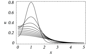
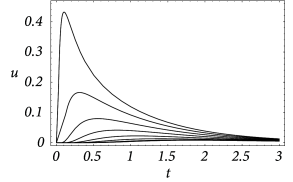
An example for the spatial distribution of the membrane potential along the cable is shown in Fig. 3.7A, where a current pulse has been injected at location $x=1$ . In addition to Fig. 3.7A, subfigure B exhibits the time course of the membrane potential measured in various distances from the point of injection. It is clearly visible that the peak of the membrane potential measured at, e.g., $x=3$ is more delayed than at, e.g., $x=2$ . Also the amplitude of the membrane potential decreases significantly with the distance from the injection point. This is a well-known phenomenon that is also present in neurons. In the absence of active amplification mechanisms, synaptic input at distal dendrites produces broader and weaker response at the soma as compared to synaptic input at proximal dendrites.

Fig. 3.7: Spatial distribution (A)and temporal evolution (B) of the membrane potential along a dendrite ( $L=5$ ) with sealed ends ( $\left.\frac{\partial}{\partial x}u\right|_{x\in\{0,L\}}=0$ ) after injection of a unit current pulse at $x=1$ and $t=0$ . The various traces in A show snapshots for time $t=0.1,\,0.2,\dots,\,1.0$ , respectively (top to bottom). The traces in B give the membrane potential as a function of time for different locations $x=1.5,\,2.0,\,2.5\dots,\,5.0$ (top to bottom) along the cable.

3.2.3 Non-linear Extensions to the Cable Equation

In the context of a realistic modeling of ‘biological’ neurons, two non-linear extensions of the cable equation have to be discussed. The obvious one is the inclusion of non-linear elements in the circuit diagram of Fig. 3.5 that account for specialized ion channels. As we have seen in the Hodgkin-Huxley model, ion channels can exhibit a complex dynamics that is in itself governed by a system of (ordinary) differential equations. The current through one of these channels is thus not simply a (non-linear) function of the actual value of the membrane potential but may also depend on the time course of the membrane potential in the past. Using the symbolic notation $i_{\text{ion}}[u](t,x)$ for this functional dependence, the extended cable equation takes the form

\frac{\partial}{\partial t}\,u(t,x)=\frac{\partial^{2}}{\partial x^{2}}\,u(t,x% )-u(t,x)-i_{\text{ion}}[u](t,x)+i_{\text{ext}}(t,x)\,.

(3.34)

A more subtle complication arises from the fact that a synapse can not be treated as an ideal current source. The effect of an incoming action potential is the opening of ion channels. The resulting current is proportional to the difference of the membrane potential and the corresponding ionic reversal potential. Hence, a time-dependent conductivity as in Eq. (3.1) provides a more realistic description of synaptic input than an ideal current source with a fixed time course.

If we replace in Eq. (3.17) the external input current $i_{\text{ext}}(t,x)$ by an appropriate synaptic input current $-i_{\text{syn}}(t,x)=-g_{\text{syn}}(t,x)[u(t,x)-E_{\text{syn}}]$ with $g_{\text{syn}}$ being the synaptic conductivity and $E_{\text{syn}}$ the corresponding reversal potential, we obtain⁴⁴We want outward currents to be positive, hence the change in the sign of $i_{\text{ext}}$ and $i_{\text{syn}}$ .

\frac{\partial}{\partial t}\,u(t,x)=\frac{\partial^{2}}{\partial x^{2}}\,u(t,x% )-u(t,x)-g_{\text{syn}}(t,x)[u(t,x)-E_{\text{syn}}]\,.

(3.35)

This is still a linear differential equation but its coefficients are now time-dependent. If the time course of the synaptic conductivity can be written as a solution of a differential equation, then the cable equation can be reformulated so that synaptic input reappears as an inhomogeneity to an autonomous equation. For example, if the synaptic conductivity is simply given by an exponential decay with time constant $\tau_{\text{syn}}$ we have

	$\displaystyle\frac{\partial}{\partial t}\,u(t,x)-\frac{\partial^{2}}{\partial x% ^{2}}\,u(t,x)+u(t,x)+g_{\text{syn}}(t,x)[u(t,x)-E_{\text{syn}}]$	$\displaystyle=0\,,$		(3.36a)
	$\displaystyle\frac{\partial}{\partial t}g_{\text{syn}}(t,x)-\tau_{\text{syn}}^% {-1}\,g_{\text{syn}}(t,x)$	$\displaystyle=S(t,x)\,.$		(3.36b)

Here, $S(t,x)$ is a sum of Dirac $\delta$ functions which describe the presynaptic spike train that arrives at a synapse located at position $x$ . Note that this equation is non-linear because it contains a product of $g_{\text{syn}}$ and $u$ which are both unknown functions of the differential equation. Consequently, the formalism based on Green’s functions can not be applied. We have reached the limit of what we can do with analytical analysis alone. To study the effect of ion channels distributed on the dendrites nummerical approaches in compartmental models become invaluable (Section 3.4).