1 Introduction 1.4 Limitations of the Leaky Integrate-and-Fire Model 1.6 Summary

1.5 What Can We Expect from Integrate-And-Fire Models?

Fig. 1.13: The challenge of spike time prediction. A current $I(t)$ is experimentally injected into the soma of a real neuron in vitro through an electrode. The response of the neuron is recorded and half of the response is made available for model optimization while part of the response remains hidden. The challenge is then to use the input $I(t)$ to predict the spike times of the hidden response with a mathematical neuron model.

The leaky integrate-and-fire model is an extremely simplified neuron model. As we have seen in the previous section, it neglects many features that neuroscientists have observed when they study neurons in the living brain or in slices of brain tissue. Therefore the question arises: what should we expect from such a model? Clearly we cannot expect it to explain the complete biochemistry and biophysics of neurons. Nor do we expect it to account for highly nonlinear interactions that are caused by active currents in some ‘hot spots’ on the dendritic tree. However, the integrate-and-fire model is surprisingly accurate when it comes to generating spikes, i.e., precisely timed events in time. Thus, it could potentially be a valid model of spike generation in neurons, or more precisely, in the soma.

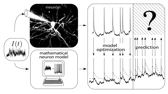
It is reasonable to require from a model of spike generation that it should be able to predict the moments in time when a real neuron spikes. Let us look at the following schematic set-up (Fig. 1.13). An experimentalist injects a time-dependent input-current $I(t)$ into the soma of a cortical neuron using a first electrode. With an independent second electrode he or she measures the voltage at the soma of the neuron. Not surprisingly, the voltage trajectory contains from time to time sharp electrical pulses. These are the action potentials or spikes.

A befriended mathematical neuroscientist now takes the time course $I(t)$ of the input current that was used by the experimentalist together with the time course of the membrane potential of the neuron and adjusts the parameters of a leaky integrate-and-fire model so that the model generates, for the very same input current, spikes at roughly the same moments in time as the real neuron. This needs some parameter tuning, but seems feasible. The relevant and much more difficult question, however, is whether the neuron model can now be used to predict the firing times of the real neuron for a novel time-dependent input current that was not used during parameter optimization (Fig. 1.13).

As discussed above, neurons not only show refractoriness after each spike but also exhibit adaptation which builds up over hundreds of milliseconds. A simple leaky integrate-and-fire model does not perform well at predicting the spike times of a real neuron. However, if adaptation (and refractoriness) is added to the neuron model, the prediction works surprisingly well. A straightforward way to add adaptation is to make the firing threshold of the neuron model dynamic: after each spike the threshold $\vartheta$ is increased by an amount $\theta$ , while during a quiescent period the threshold approaches its stationary value $\vartheta_{0}$ . We can use the Dirac $\delta$ -function to express this idea

\tau_{\rm adapt}{{\text{d}}\over{\text{d}}t}\vartheta(t)=-[\vartheta(t)-% \vartheta_{0}]+\theta\sum_{f}\delta(t-t^{(f)})

(1.34)

where $\tau_{\rm adapt}$ is the time constant of adaptation (a few hundred milliseconds) and $t^{(f)}=t^{(1)},t^{(2)},t^{(3)}...$ are the firing times of the neuron.

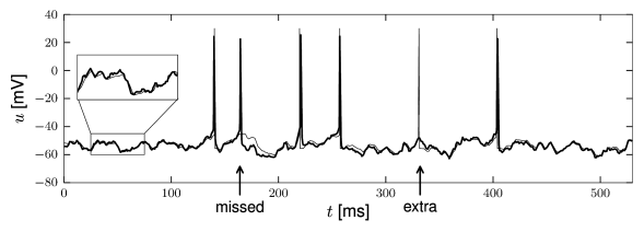
The predictions of an integrate-and-fire model with adaptive threshold agree nicely with the voltage trajectory of a real neuron, as can be seen from Fig. 1.14. The problem of how to construct practical, yet powerful, generalizations of the simple leaky integrate-and-fire model is the main topic of Part II of the book. Another question arising from this is how to quantify the performance of such neuron models (see Chapters 11).

Fig. 1.14: Comparing a generalized integrate-and-fire model with experimental traces. A voltage trace (thick black trace) recorded in a real neuron driven by a fluctuating current is superposed on the voltage trace generated by a generalized integrate and fire model (thin line) driven by the same current. The subthreshold voltage fluctuations are accurately predicted (inset) and the spike timings are well predicted on average, apart from a few additional or missed spikes (arrows).

Once we have identified good candidate neuron models, we will ask in Part III, whether we can construct big populations of neurons with these models, and whether we can use them to understand the dynamic and computational principles as well as potential neural codes used by populations of neurons. Indeed, as we will see, it is possible to make the transition from plausible single-neuron models to large and structured populations. This does not mean that we understand the full brain, but understanding the principles of large populations of neurons from well-tested simplified neuron models is a first and important step in this direction.