16 Competing Populations and Decision Making 16.3 Dynamics of decision making 16.5 Human Decisions, Determinism, and Free Will

16.4 Alternative Decision Models

In the previous two sections, we discussed decision models as the competitive interaction between two or more populations of excitatory neurons. In this section we present two different models of decision making, i.e., the energy picture in subsection 16.4.1 and the drift-diffusion model in subsection 16.4.2. Both models are phenomenological concepts to describe decision making. However, both models are also related to the phase diagram of the model of two neuronal populations, encountered in Section 16.3.

Fig. 16.9: Energy picture of decision making. A. Decisions correspond to a ball rolling down an energy landscape, plotted as a function of a formal decision variable $x$ . A value of $x=0$ indicates that no decision is taken (top, no input), whereas a value of $x=\pm 1$ reflects a decision for options A or B, respectively. An input favoring option A deforms and tilts the energy landscape so that the minimum of the energy is in the neighborhood of $x=1$ (middle). A strong but unbiased input, creates two energy minima corresponding to options A and B. Only one of the two options can be taken by the rolling ball (bottom). B. The corresponding phase plane diagram of the input potentials $h_{A}$ (horizontal axis) and $h_{B}$ (vertical axis). Fixed points are indicated as filled (stable) or empty (saddle) circles. The decision variable $x$ moves along the axis (short-dashed gray line) perpendicular to the diagonal (long-dashed black line) and is replotted again as a one-dimensional flow on the right-hand side of the figure.

16.4.1 The energy picture

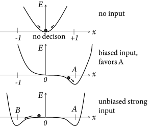
Binary decisions can be visualized as a ball in a hilly energy landscape. Once the ball rolls in a certain direction, a decision starts to form. The decision is finalized when the ball approaches the energy minimum; cf. Fig. 16.9A. The decision variable $x$ reflects a decision for option A, if it approaches a fixed point in the neighborhood of $x\approx 1$ and a decision for option B for $x\approx-1$ . If the variable $x$ is trapped in a minimum close to $x=0$ , no decision is taken.

The dynamics of the decision process can be formulated as gradient descent

{dx\over dt}=-\eta{dE\over dx}

(16.11)

with a positive constant $\eta$ . In other words, in a short time step $\Delta t$ , the decision variable moves by an amount $-\eta\Delta t\,dE/dx$ . Thus, if the slope is positive, the movement is toward the left. As a result, the movement is always downhill, so that the energy decreases along the trajectory $x(t)$ . We can calculate the change of the energy along the trajectory

{dE(x(t))\over dt}={dE\over dx}\,{dx\over dt}=-\eta\left({dE\over dx}\right)^{% 2}\leq 0\,.

(16.12)

Therefore the energy plays the role of a Liapunov function of the system, i.e., a quantity that cannot increase along the trajectory of a dynamical system .

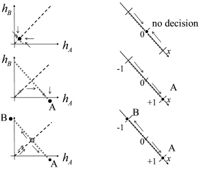
Interestingly, the energy picture can be related to the phase plane analysis of the two-dimensional model that we encountered earlier in Figs. 16.6B and 16.7. The diagonal of the phase plane plays the role of the boundary between the options A and B while the variable $x$ indicates the projection onto an axis orthogonal to the diagonal. $x=0$ is the unbiased, undecided position on the diagonal; cf. Fig. 16.9. In the case of strong unbiased input, the one-dimensional flow diagram of the variable $x$ presents a reasonable summary of the flow pattern in the two-dimensional system, because the saddle point in the phase plane is attractive along the diagonal and is reached rapidly while the flow in the perpendicular direction is much slower (543; 61; 558).

The above arguments regarding the Liapunov function of the network can be made more precise and formulated as general theorem (100; 227). We consider an arbitrary network of $K$ neuronal population $1\leq j\leq K$ with population rate $A_{j}=g(h_{j})\geq 0$ where $g$ is a gain function with derivative $g^{\prime}>0$ and $h$ follows the dynamics

\tau\,{{\text{d}}h_{j}\over{\text{d}}t}=-h_{j}+R\,I_{j}\,+\sum_{k}w_{jk}g(h_{k% })\,

(16.13)

with fixed inputs $I_{j}$ . If the coupling is symmetric, i.e., $w_{ij}=w_{ji}$ then the energy

E=-\sum_{i}\sum_{j}w_{ij}A_{i}A_{j}-\sum_{i}A_{i}\,R\,I_{i}+\sum_{i}\int_{0}^{% A_{i}}g^{-1}(a)\,{\text{d}}a\,

(16.14)

is a Liapunov function of the dynamics.

The proof follows by taking the derivative. We exploit the fact that $w_{ij}=w_{ji}$ and apply the chain rule $dA_{i}/dt=g^{\prime}(h_{i})dh_{i}/dt$ so as to find

	$\displaystyle{dE\over dt}$	$\displaystyle=$	$\displaystyle-\sum_{i}\left[\sum_{j}w_{ij}A_{j}\right]\,g^{\prime}(h_{i}){dh_{% i}\over dt}-\sum_{i}R\,I_{i}\,g^{\prime}(h_{i}){dh_{i}\over dt}+\sum_{i}g^{-1}% (A_{i})\,g^{\prime}(h_{i}){dh_{i}\over dt}$		(16.15)
		$\displaystyle=$	$\displaystyle-\tau\sum_{i}g^{\prime}(h_{i})\left[{dh_{i}\over dt}\right]^{2}% \leq 0\,.$		(16.15)

In the second line we have used Eq. (16.13). Furthermore, since the neuronal gain function stays below a biologically sustainable firing rate $g(x)\leq A^{\rm max}$ , the energy is bounded from below. Therefore the flow of a symmetric network of interacting populations will always converge to one of the stable fixed points corresponding to an energy minimum, – unless the initial condition is chosen to lie on an unstable fixed point in which case the dynamics stays there until it is perturbed by some input.

Example: Binary decision network revisited

The binary decision network of Eqs. (16.7) and (16.8) with effective inhibition $\alpha$ and recurrent interactions $w_{0}$ consists of two populations. Interactions are symmetric since $w_{12}=w_{21}=-\alpha$ . Therefore the energy function

E=-w_{0}[A_{1}^{2}+A_{2}^{2}]+2\alpha A_{1}A_{2}-R\,[I_{1}A_{1}+I_{2}A_{2}]+% \int_{0}^{A_{1}}g^{-1}(x)dx+\int_{0}^{A_{2}}g^{-1}(y)dy

(16.16)

is a Liapunov function of the dynamics defined in Eqs. (16.7) and (16.8). Since the dynamics is bounded, there must be stable fixed points.

16.4.2 Drift-Diffusion Model

Fig. 16.10: Drift-diffusion model. The decision variable $x(t)$ starts from $x_{0}$ and undergoes a biased random walk toward one of the two thresholds, marked by horizontal dashed lines. In the first trial (thin solid line), the choice is option $A$ and the reaction time indicated as $t_{A}$ . In another trial (thick solid line) the trajectory hits, after a time $t_{B}$ the threshold for option B.

The drift-diffusion model is a phenomenological model to describe choice preferences and distributions of reaction times in binary decision making tasks (422). At each trial of a decision experiment, a decision variable $x$ is initialized at time $t_{0}$ at a value $x(t_{0})=x_{0}$ . Thereafter, the decision variable evolves according to

{dx\over dt}=(I_{A}-I_{B})+\sigma\xi(t)

(16.17)

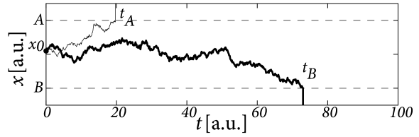
where $\xi(t)$ is Gaussian white noise of unit mean and variance $\sigma^{2}$ . An input $I_{A}>I_{B}$ causes a ‘drift’ of the variable $x$ toward positive values while the noise $\xi$ leads to a ‘diffusion’-like motion of the trajectory; hence the name ‘drift-diffusion model’.

The reaction time is the time at which the variable $x$ reaches one of two thresholds, $\Theta_{A}$ or $\Theta_{B}$ , respectively (Fig. 16.10). For example $t_{B}$ defined by $t_{B}={\rm min}\left\{t|x(t)=\Theta_{B}\right\}$ is the reaction time in a trial where the choice falls on option $B$ .

Parameters of the phenomenological drift-diffusion model are the values of thresholds $\Theta_{A}$ and $\Theta_{B}$ , and the strength of the input $I_{A}-I_{B}$ compared to that of the noise. The initial condition $x_{0}$ can be identical in all trials or chosen in each trial independently from a small interval that reflects uncontrolled variations in the bias of the subject. The time $t_{0}$ is typically the moment when the subject receives the choice stimulus, but it is also possible to start the drift-diffusion process a few milliseconds later so as to account for the propagation delay from the sensors to the brain (422; 421).

Example: Drift-diffusion model versus neuronal models

In the original formulation, the drift-diffusion model was used as a ‘black box’, i.e., a phenomenological model with parameters that can be fitted to match the distribution of reaction times and choice preferences to behavioral experiments. Interestingly, however, variants of one-dimensional drift-diffusion models can be derived from the models of neural populations with competitive interaction that we have discussed in earlier sections of this chapter (61; 558; 447). The essential idea can be best explained in the energy picture; cf. Fig. 16.9. We assume a small amount of noise. In the absence of input, the decision variable jitters around the stable fixed point $x=0$ . Its momentary value $x\approx 0$ serves as an initial condition, once the input is switched on. Suppose the input is strong but unbiased. Two new valleys form around $x\approx\pm 1$ . However, in the neighborhood of $x=0$ the landscape is flat, so that noise leads to a diffusive motion of the trajectory. A biased input $I_{A}>I_{B}$ tilts the energy landscape to the right which causes a corresponding drift term in the diffusion process. The location where the slope of the valley becomes steep can be associated with the threshold $\Theta_{A}$ in the diffusion model.