7 Variability of Spike Trains and Neural Codes 7.5 Renewal statistics 7.7 Summary

7.6 The Problem of Neural Coding

We have discussed in the preceding sections measures to quantify neural spike train data. This includes measures of interval distribution, autocorrelation, noise spectrum, but also simple measures such as the firing rate. All of these measures are useful tools for an experimenter who plans to study a neural system. A completely different question, however, is whether neurons transmit information by using any of these quantities as a neural code.

In this section we critically review the notion of rate codes, and contrast rate coding schemes with spike codes.

7.6.1 Limits of rate codes

The successful application of rate concepts to neural data does not necessarily imply that the neuron itself uses a rate code. Let us look at the limitations of the spike count measure and the PSTH.

Limitations of the spike count code. An experimenter as an external observer can evaluate and classify neuronal firing by a spike count measure – but is this really the code used by neurons in the brain? In other words, is a cortical neuron which receives signals from a sensory neuron only looking at and reacting to the number of spikes it receives in a time window of, say, 500 ms? We will approach this question from a modeling point of view later on in the book. Here we discuss some critical experimental evidence.

From behavioral experiments it is known that reaction times are often rather short. A fly can react to new stimuli and change the direction of flight within 30-40 ms; see the discussion in (436). This is not long enough for counting spikes and averaging over some long time window. The fly has to respond after a postsynaptic neuron has received one or two spikes. Humans can recognize visual scenes in just a few hundred milliseconds (512), even though recognition is believed to involve several processing steps. Again, this does not leave enough time to perform temporal averages on each level.

From the point of view of rate coding, spikes are just a convenient way to transmit the analog output variable $\nu$ over long distances. In fact, the best coding scheme to transmit the value of the rate $\nu$ would be by a regular spike train with intervals $1/\nu$ . In this case, the rate could be reliably measured after only two spikes. From the point of view of rate coding, the irregularities encountered in real spike trains of neurons in the cortex must therefore be considered as noise. In order to get rid of the noise and arrive at a reliable estimate of the rate, the experimenter has to average over a larger number of spikes.

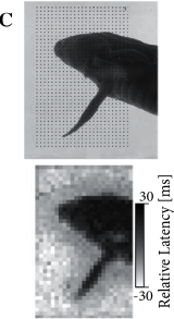
Temporal averaging can work well in cases where the stimulus is constant or slowly varying and does not require a fast reaction of the organism - and this is the situation encountered in many experimental protocols. Real-world input, however, is rarely stationary, but often changing on a fast time scale. For example, even when viewing a static image, humans perform saccades, rapid changes of the direction of gaze. The image projected onto the retinal photo receptors changes therefore every few hundred milliseconds - and with each new image the retinal photo receptors change the response (Fig. 7.16C). Since, in a changing environment, a postsynaptic neuron does not have the time to perform a temporal average over many (noisy) spikes, we consider next whether the PSTH could be used by a neuron to estimate a time-dependent firing rate.

Limitations of the PSTH. The obvious problem with the PSTH is that it needs several trials to build up. Therefore it can not be the decoding scheme used by neurons in the brain. Consider for example a frog which wants to catch a fly. It can not wait for the insect to fly repeatedly along exactly the same trajectory. The frog has to base its decision on a single run – each fly and each trajectory is different.

Nevertheless, the PSTH measure of the instantaneous firing rate can make sense if there are large populations of similar neurons that receive the same stimulus. Instead of recording from a population of $N$ neurons in a single run, it is experimentally easier to record from a single neuron and average over $N$ repeated runs. Thus, a neural code based on the PSTH relies on the implicit assumption that there are always populations of neurons with similar properties.

Limitations of rate as a population average. A potential difficulty with the definition (7.11) of the firing rate as an average over a population of neurons is that we have formally required a homogeneous population of neurons with identical connections which is hardly realistic. Real populations will always have a certain degree of heterogeneity both in their internal parameters and in their connectivity pattern. Nevertheless, rate as a population activity (of suitably defined pools of neurons) may be a useful coding principle in many areas of the brain.

For inhomogeneous populations, the definition (7.11) may be replaced by a weighted average over the population. In order to give an example of a weighted average in an inhomogeneous population, we suppose that we are studying a population of neurons which respond to a stimulus ${\bf x}$ . We may think of ${\bf x}$ as the location of the stimulus in input space. Neuron $i$ responds best to stimulus ${\bf x}_{i}$ , another neuron $j$ responds best to stimulus ${\bf x}_{j}$ . In other words, we may say that the spikes of a neuron $i$ ‘represent’ an input vector ${\bf x}_{i}$ and those of $j$ an input vector ${\bf x}_{j}$ . In a large population, many neurons will be active simultaneously when a new stimulus ${\bf x}$ is represented. The location of this stimulus can then be estimated from the weighted population average

{\bf x}^{\rm est}(t)={\int_{t}^{t+\Delta t}\sum_{j}\sum_{f}{\bf x}_{j}\,\delta% (t-t_{j}^{(f)})\,dt\over\int_{t}^{t+\Delta t}\sum_{j}\sum_{f}\,\delta(t-t_{j}^% {(f)})\,{\text{d}}t}\,.

(7.52)

Both numerator and denominator are closely related to the population activity (7.11). The estimate (7.52) has been successfully used for an interpretation of neuronal activity in primate motor cortex (171) and hippocampus (554). It is, however, not completely clear whether postsynaptic neurons really evaluate the fraction (7.52) – a potential problem for a neuronal coding and decoding scheme lies in the normalization by division.

Fig. 7.15: Time-to-first spike. The spike train of three neurons are shown. The third neuron from the top is the first one to fire a spike after the stimulus onset (arrow). The dashed line indicates the time course of the stimulus.

7.6.2 Candidate temporal codes

Rate coding in the sense of a population average is one of many candidate coding schemes that could be implemented and used by neurons in the brain. In this section, we introduce some potential coding strategies based on spike timing.

Time-to-first-spike: Latency code

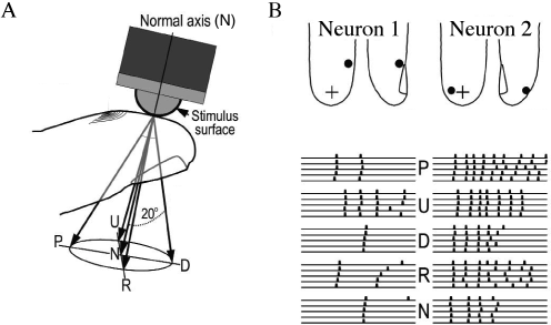
Let us study a neuron which abruptly receives a new constant input at time $t_{0}$ . For example, a neuron might be driven by an external stimulus which is suddenly switched on at time $t_{0}$ . This seems to be somewhat artificial, but even in a realistic situation abrupt changes in the input are quite common. When we look at a picture, our gaze jumps from one point to the next. After each saccade, the photo receptors in the retina receive a new visual input. Information about the onset of a saccades should easily be available in the brain and could serve as an internal reference signal. We can then imagine a code where for each neuron the timing of the first spike after the reference signal contains all information about the new stimulus. A neuron which fires shortly after the reference signal is interpreted as a strong stimulation of this neuron, whereas firing somewhat later would signal a weaker stimulation; see Fig. 7.15.

Fig. 7.16: Time-to-first-spike. A. Touching the finger tip with a sharp object can be quantified by a force vector with total strength in normal direction (N), possibly superimposed with a tangential component in one of four possible directions (P,U,D,R). B. Spike response to onset of touch force in the five possible direction (P,U,D,R,N). Different stimuli yield different spike latencies which are consistent across the 5 repetitions. Different neurons have different response patterns (two selected neurons are shown). The location where stimulation yields maximal response is shown with a filled circle. C. (Top) Presentation of an image on the retina. The grid of recording electrodes is indicated by dots. (Bottom) The latency of the first spike detected at each electrode reflects the original image. Each pixel corresponds to one recorded neuron. A and B modified from Johansson and Birznieks (244), C modified from Gollisch and Meister (194).

In a pure version of this coding scheme, each neuron only needs to fire a single spike to transmit information. If it emits several spikes, only the first spike after the reference signal counts. All following spikes would be irrelevant. To implement a clean version of such a coding scheme, we imagine that each neuron is shut off by inhibition as soon as it has fired a spike. Inhibition ends with the onset of the next stimulus (e.g., after the next saccade). After the release from inhibition the neuron is ready to emit its next spike that now transmits information about the new stimulus. Since each neuron in such a scenario transmits exactly one spike per stimulus, it is clear that only the timing conveys information and not the number of spikes.

Experimental evidences indicate that a coding scheme based on the latency of the first spike transmit a large amount of information. For example touch sensors in the finger tip encode the strength and direction of the touch in the timing of the first spike emitted by each neuron (Fig. 7.16). Similarly, the relative latency of first spikes of retinal neurons encode the image projected on the retina (Fig. 7.16C). In a slightly different context coding by first spikes has been discussed by S. Thorpe (512). Thorpe argues that the brain does not have time to evaluate more than one spike from each neuron per processing step. Therefore the first spike should contain most of the relevant information, which is read out by neurons further down the processing chain. Using information-theoretic measures on their experimental data, several groups have shown that most of the information about a new stimulus is indeed conveyed during the first 20 or 50 milliseconds after the onset of the neuronal response (372; 517).

Phase

We can apply a code by ’time to first spike’ also in the situation where the reference signal is not a single event, but a periodic signal. In the hippocampus, in the olfactory system, and also in other areas of the brain, oscillations of some global variable (for example the population activity) are quite common. These oscillations could serve as an internal reference signal. Neuronal spike trains could then encode information in the phase of a pulse with respect to the background oscillation. If the input does not change between one cycle and the next, then the same pattern of phases repeats periodically; see Fig. 7.17A.

The concept of coding by phases has been studied by several different groups. There is, for example, evidence that the phase of a spike during an oscillation in the hippocampus of the rat conveys information on the spatial location of the animal which is not fully accounted for by the firing rate of the neuron (375).

Correlations and Synchrony

We can also use spikes from other neurons as the reference signal for a spike code. For example, synchrony of a pair or of many neurons could signify special events and convey information which is not contained in the firing rate of the neurons; see Fig. 7.17B. One famous idea is that synchrony could mean ‘belonging together’. Consider for example a complex scene consisting of several objects. It is represented in the brain by the activity of a large number of neurons. Neurons which represent the same object could be ‘labeled’ by the fact that they fire synchronously (541; 134; 197).

More generally, not only synchrony but any precise spatio-temporal pulse pattern could be a meaningful event. For example, a spike pattern of three neurons, where neuron 1 fires at some arbitrary time $t_{1}$ followed by neuron 2 at time $t_{1}+\delta_{12}$ and by neuron 3 at $t_{1}+\delta_{13}$ , might represent a certain stimulus condition. The same three neurons firing with different relative delays might signify a different stimulus. The relevance of precise spatio-temporal spike patterns has been studied intensively by Abeles (7). Similarly, but on a somewhat coarse time scale, correlations of auditory and visual neurons are found to be stimulus dependent and might convey information beyond that contained in the firing rate alone (119; 497).

Stimulus Reconstruction and Reverse Correlation

Let us consider a neuron which is driven by a time dependent stimulus $s(t)$ . Every time a spike occurs, we note the time course of the stimulus in a time window of about 100 milliseconds immediately before the spike. Averaging the results over several spikes yields the typical time course of the stimulus just before a spike (113). Such a procedure is called a ‘reverse correlation’ approach; see Fig. 7.18. In contrast to the PSTH experiment sketched in Section 7.2.2 where the experimenter averages the neuron’s response over several trials with the same stimulus, reverse correlation means that the experimenter averages the input under the condition of an identical response, that is, a spike. In other words, it is a spike-triggered average; see, e.g., (114; 436). The results of the reverse correlation, i.e., the typical time course of the stimulus which has triggered a spike, can be interpreted as the ‘meaning’ of a single spike. Reverse correlation techniques have made it possible to measure, for example, the spatio-temporal characteristics of neurons in the visual cortex (135; 116).

Fig. 7.18: Reverse correlation technique (schematic). The stimulus in the top trace has caused the spike train shown immediately below. The time course of the stimulus just before the spikes (dashed boxes) has been averaged to yield the typical time course (bottom).

With a somewhat more elaborate version of this approach, W. Bialek and his co-workers have been able to ‘read’ the neural code of the H1 neuron in the fly and to reconstruct a time-dependent stimulus (57; 436). Here we give a simplified version of their argument.

Results from reverse correlation analysis suggest that each spike signifies the time course of the stimulus preceding the spike. If this is correct, a reconstruction of the complete time course of the stimulus $s(t)$ from the set of firing times ${\mathcal{F}}=\{t^{(1)},\dots t^{(n)}\}$ should be possible; see Fig. 7.19. As a simple test of this hypothesis, Bialek and coworkers have studied a linear reconstruction. A spike at time $t^{(f)}$ gives a contribution $\kappa(t-t^{(f)})$ to the estimation $s^{\rm est}(t)$ of the time course of the stimulus. Here, $t^{(f)}\in{\mathcal{F}}$ is one of the firing times and $\kappa(t-t^{(f)})$ is a kernel which is nonzero during some time before and around $t^{(f)}$ ; cf. Fig. 7.19B. A linear estimate of the stimulus is

s^{\rm est}(t)=\sum_{f=1}^{n}\kappa(t-t^{(f)})\,.

(7.53)

The form of the kernel $\kappa$ was determined through optimization so that the average reconstruction error $\int{\text{d}}t[s(t)-s^{\rm est}(t)]^{2}$ was minimal. The quality of the reconstruction was then tested on additional data which was not used for the optimization. Surprisingly enough, the simple linear reconstruction (7.53) gave a fair estimate of the time course of the stimulus even though the stimulus varied on a time scale comparable to the typical interspike interval (57; 436). This reconstruction method shows nicely that information about a time dependent input can indeed be conveyed by spike timing. Chapter 11 will revisit the spike train decoding in the presence of refractoriness and adaptation.

Fig. 7.19: Reconstruction of a stimulus (schematic). A. A stimulus evokes a spike train of a neuron. The time course of the stimulus may be estimated from the spike train; redrawn after [Rieke et al., 1996]. B. In the framework of linear stimulus reconstruction, the estimation $s^{\rm est}(t)$ (dashed) is the sum of the contributions $\kappa$ (solid lines) of all spikes.

Rate versus temporal codes (*)

The dividing line between spike codes and firing rates is not always as clearly drawn as it may seem at first sight. Some codes which were first proposed as pure examples of pulse codes have later been interpreted as variations of rate codes. For example the stimulus reconstruction (7.53) with kernels seems to be a clear example of a spike code. Nevertheless, it is also not so far from a rate code based on spike counts (6; 510). To see this, consider a spike count measure with a running time window $K(.)$ . We can estimate the rate $\nu$ at time $t$ by

\nu(t)={\int K(\tau)\,S(t-\tau)d\tau\over\int K(\tau)d\tau}\,,

(7.54)

where $S(t)=\sum_{f=1}^{n}\delta(t-t^{(f)})$ is the spike train under consideration. The integrals run from minus to plus infinity. For a rectangular time window $K(\tau)=1$ for $-T/2<\tau<T/2$ and zero otherwise, (7.54) reduces exactly to our definition (7.1) of a rate as a spike count measure in Eq. (7.1).

The time window in (7.54) can be made rather short so that at most a few spikes fall into the interval $T$ . Furthermore, there is no need that the window $K(.)$ be symmetric and rectangular. We may just as well take an asymmetric time window with smooth borders. Moreover, we can perform the integration over the $\delta$ function which yields

\nu(t)=c\,\sum_{f=1}^{n}K(t-t^{(f)})

(7.55)

where $c=[\int K(s)ds]^{-1}$ is a constant. Except for the constant $c$ (which sets the overall scale to units of one over time), the generalized rate formula (7.55) is now identical to the reconstruction formula (7.53). In other words, the linear reconstruction is just the firing rate measured with a cleverly optimized time window.

Similarly, a code based on the ‘time-to-first-spike’ is also consistent with rate coding. If, for example, the mean firing rate of a neuron is high for a given stimulus, then the first spike is expected to occur early. If the rate is low, the first spike is expected to occur later. Thus the timing of the first spike contains a lot of information about the underlying rate.

The discussion of whether or not to call a given code a rate code is still ongoing. What is important, in our opinion, is to have a coding scheme which allows neurons to quickly respond to stimulus changes. A naïve spike count code with a long time window is unable to do this, but a code based on population activities introduced above and many of the other codes are. The name of such a code, whether it is deemed a rate code or not is of minor importance.

Example: Towards a definition of rate codes

We have seen above in Eq. (7.55) that stimulus reconstruction with a linear kernel can be seen as a special instance of a rate code. This suggests a formal definition of a rate code via the reconstruction procedure: if all information contained in a spike train can be recovered by the linear reconstruction procedure of Eq. (7.53), then the neuron is, by definition, using a rate code. Spike codes would then be codes where a linear reconstruction is not successful. Theunissen and Miller have proposed a definition of rate coding that makes the above ideas more precise (510).

To see how their definition works, we have to return to the reconstruction formula (7.53). It is, in fact, the first term of a systematic Volterra expansion for the estimation of the stimulus from the spikes (57)

s^{\rm est}(t)=\sum_{f}\kappa_{1}(t-t^{(f)})\,+\sum_{f,f^{\prime}}\kappa_{2}(t% -t^{(f)},t-t^{(f^{\prime})})\,+\dots\,.

(7.56)

For a specific neuron, inclusion of higher-order terms $\kappa_{2},\kappa_{3},\dots$ may or may not improve the quality of the estimation. For most neurons where the reconstruction has been carried through, it seems that the higher-order terms do not contribute a large amount of information (436). The neurons would then be classified as rate coding.

Let us now suppose that the reconstruction procedure indicates a significant contribution of the second-order term. Does this exclude rate coding? Unfortunately this is not the case. We have to exclude two other possibilities. Firstly, we might have chosen a suboptimal stimulus. A neuron might for example encode the variable $x$ by a rate code, so that a nearly perfect linear reconstruction of $x$ would be possible,

x(t)\approx x^{\rm est}=\sum_{f=1}^{n}\kappa_{1}(t-t^{(f)})\,;

(7.57)

But if we chose a stimulus $s=x^{2}$ instead of $x$ , then the reconstruction for $s^{\rm est}$ would involve second-order terms, even though the neuron is really using rate code.

Secondly, according to Theunissen and Miller [1995] a spike code should show a temporal structure that is more precise than the temporal structure of the stimulus. The fact that neurons show precise and reliable spike timing as such is, for them, not sufficient to classify the neuron as a temporal encoder, since the neuronal precision could just be the image of precise temporal input. For a more quantitative treatment, let us consider a stimulus with cut-off frequency $\omega$ . In order to exclude the possibility that the timing is induced by the stimulus, Theunissen and Miller propose to consider the Fourier spectrum of the higher-order reconstruction kernels. If the Fourier transform of the higher-order kernels contains frequencies less than $\omega$ only, then the code is a rate code. If higher-order kernels are significant and contain frequencies above $\omega$ , then the information is encoded temporally. A positive example of a spike code (or of ‘temporal encoding’) according to this definition would be the code by correlation and synchrony introduced above. Another example would be the phase code, in particular if the number of spikes per cycle is independent of the stimulus strength.