8 Noisy Input Models: Barrage of Spike Arrivals 8 Noisy Input Models: Barrage of Spike Arrivals 8.2 Stochastic spike arrival

8.1 Noise input

Neurons are driven by an input current $I(t)$ which summarizes the effect of synaptic input from other neurons in the network in vivo or the current injected by an experimenter into a cell in vitro. Modeling the noisiness of the input amounts to splitting the input current into two components, a deterministic and a stochastic one

I(t)=I^{\rm det}(t)+I^{\rm noise}(t)\,,

(8.1)

where the deterministic term $I^{\rm det}$ summarizes the part of the current which is known, or at least predictable, while the stochastic term $I^{\rm noise}$ is the unpredictable, or noisy, part of the current.

For example, during an in vitro study with intracellular current injection, $I^{\rm det}$ would be the current that is set on the switchboard of the current generator, but the actual current fluctuates around the preset value because of finite temperature. In a neural recording during a visual psychophysics experiment in vivo, the part of the input current that does not change across trials with the same visual stimulus would be summarized as $I^{\rm det}$ , while all the remaining inputs to the neuron which vary from one trial to the next are treated as noise and summarized as $I^{\rm noise}$ .

For modeling, the noise term is simply added on the right-hand side of the differential equation of the voltage. For example, a nonlinear integrate-and-fire model with noisy input has the voltage equation

\tau_{m}{{\text{d}}\over{\text{d}}t}u=f(u)+R\,I^{\rm det}(t)+R\,I^{\rm noise}(% t)\,.

(8.2)

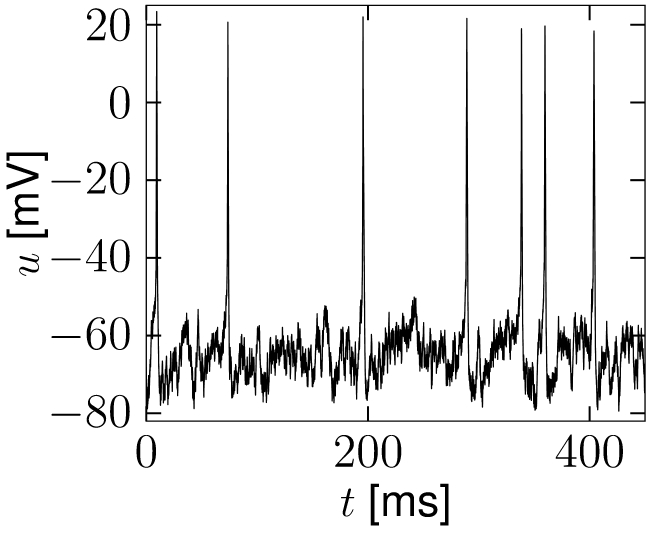
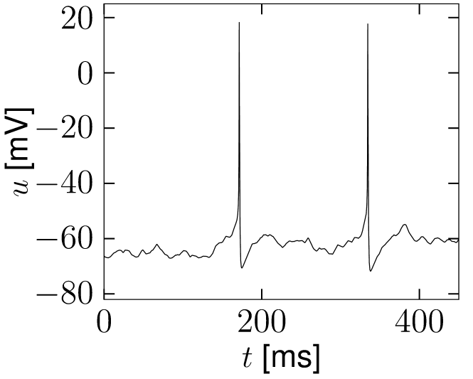
If $u$ reaches the threshold $\theta_{\rm reset}$ , the integration is stopped and the membrane potential reset to $u_{r}$ . The procedure of adding input noise is completely analogous for biophysical models of the Hodgkin-Huxley type or integrate-and-fire models with adaptation; see Fig. 8.1.

Fig. 8.1: Noisy input. A. A Hodgkin-Huxley model with parameters as in Chapter 2 driven with white-noise input. B. The same model driven with colored noise with time constant $\tau_{s}=50$ ms. Note that the fluctuations of the membrane potential are slower.

8.1.1 White noise

The standard procedure of implementing the noise term $R\,I^{\rm noise}$ in the differential equation of the membrane voltage is to formulate it as a ‘white noise’, $R\,I^{\rm noise}(t)=\xi(t)$ . White noise $\xi$ is a stochastic process characterized by its expectation value,

\langle\xi(t)\rangle=0\,,

(8.3)

and the autocorrelation

\langle\xi(t)\,\xi(t^{\prime})\rangle=\sigma^{2}\,\tau_{m}\,\delta(t-t^{\prime% })\,,

(8.4)

where $\sigma$ is the amplitude of the noise (in units of voltage) and $\tau_{m}$ the time constant of the differential equation (8.2). Eq. (8.4) indicates that the process $\xi$ is uncorrelated in time: knowledge of the value $\xi$ at time $t$ does not enable us to predict its value at any other time $t^{\prime}\neq t$ . The Fourier transform of the autocorrelation function (8.4) yields the power spectrum; cf. Section 7.4. The power spectrum of white noise is flat, i.e., the noise is equally strong at all frequencies.

If the white noise term is added on the right-and-side of (8.2), we arrive at a stochastic differential equation, i.e., an equation for a stochastic process,

\tau_{m}\frac{{\text{d}}}{{\text{d}}t}u(t)=f(u(t))+R\,I^{\rm det}(t)+\xi(t)\,,

(8.5)

also called Langevin equation. In Section 8.2 we will indicate how the noise term $\xi(t)$ can be derived from a model of stochastic spike arrival.

In the mathematical literature, instead of a ’noise term’ $\xi(t)$ , a different style of writing the Langevin equation dominates. To arrive at this alternative formulation we first divide both sides of Eq. (8.5) by $\tau_{m}$ and then multiply with the short time step ${\text{d}}t$ ,

{\text{d}}u=f(u)\,{{\text{d}}t\over\tau_{m}}+R\,I^{\rm det}(t)\,{{\text{d}}t% \over\tau_{m}}+\sigma{\text{d}}W_{t},

(8.6)

where ${\text{d}}W_{t}$ are the increments of the Wiener process in a short time ${\text{d}}t$ , that is, ${\text{d}}W_{t}$ are random variables drawn from a Gaussian distribution with zero mean and variance proportional to the step size ${\text{d}}t$ . This formulation therefore has the advantage that it can be directly used for simulations of the model in discrete time. White noise which is Gaussian distributed is called Gaussian white noise. Note for a numerical implementation of Eq. (8.6) that it is the variance of the Gaussian which is proportional to the step size; therefore its standard deviation is proportional to $\sqrt{{\text{d}}t}$ .

Example: Leaky integrate-and-fire model with white noise input

In the case of the leaky integrate-and-fire model (with voltage scale chosen such that the resting potential is at zero), the stochastic differential equation is

\tau_{m}\frac{{\text{d}}}{{\text{d}}t}u(t)=-u(t)+R\,I^{\rm det}(t)+\xi(t)\,,

(8.7)

which is called the Ornstein-Uhlenbeck process (527; 529).

We note that the white noise term on the right-and-side is integrated with a time constant $\tau_{m}$ to yield the membrane potential. Therefore fluctuations of the membrane potential have an autocorrelation with characteristic time $\tau_{m}$ . We will refer to Eq. (8.7) as the Langevin equation of the noisy integrate-and-fire model.

A realization of a trajectory of the noisy integrate-and-fire model defined by Eq. (8.7) is implemented in discrete time by the iterative update

{\text{d}}u=(-u+R\,I^{\rm det}){{\text{d}}t\over\tau_{m}}+\sigma\sqrt{{\text{d% }}t}\,y,

(8.8)

where $y$ is a random number drawn from a zero-mean Gaussian distribution of unit variance (i.e., ${\text{d}}W=\sqrt{{\text{d}}t}\,y$ has variance proportional to ${\text{d}}t$ ). Note that for small step size ${\text{d}}t$ and finite current amplitude $I^{\rm det}$ , the voltage steps ${\text{d}}u$ are small as well so that, despite the noise, the trajectory becomes smooth in the limit of ${\text{d}}t\to 0$ .

A noisy integrate-and-fire neuron is said to fire an action potential whenever the membrane potential $u$ updated via (8.8) reaches the threshold $\vartheta$ ; cf. Fig. 8.2. The analysis of Eq. (8.7) in the presence of the threshold $\vartheta$ is one of the major topics of this chapter. Before turning to the problem with threshold, we determine now the amplitude of membrane potential fluctuations in the absence of a threshold.

Fig. 8.2: Noisy integration. A stochastic contribution in the input current of an integrate-and-fire neuron causes the membrane potential to drift away from the reference trajectory (thick solid line). The neuron fires if the noisy trajectory (thin line) hits the threshold $\vartheta$ .

8.1.2 Noisy versus noiseless membrane potential

The Langevin equation of the leaky integrate-and-fire model with white noise input is particularly suitable to compare the membrane potential trajectory of a noisy neuron model with that of a noiseless one.

Let us consider Eq. (8.7) for constant $\sigma$ . At $t=\hat{t}$ the membrane potential starts at a value $u=u_{r}=0$ . Since (8.7) is a linear equation, its solution for $t>\hat{t}$ is

u(t)={R\over\tau_{m}}\int_{0}^{t-\hat{t}}e^{-s/\tau_{m}}\,I^{(\rm det)}(t-s)\,% {\text{d}}s\,+{1\over{\tau_{m}}}\int_{0}^{t-\hat{t}}\,e^{-s/\tau_{m}}\,\xi(t-s% )\,{\text{d}}s.

(8.9)

Since $\langle\xi(t)\rangle=0$ , the expected trajectory of the membrane potential is

u_{0}(t)=\langle u(t|\hat{t})\rangle={R\over\tau_{m}}\int_{0}^{t-\hat{t}}e^{-s% /\tau_{m}}\,I^{(\rm det)}(t-s)\,{\text{d}}s\,.

(8.10)

In particular, for constant input current $I^{(\rm det)}(t)\equiv I_{0}$ we have

u_{0}(t)=u_{\infty}\,\left[1-e^{-(t-\hat{t})/\tau_{m}}\right]\,

(8.11)

with $u_{\infty}=R\,I_{0}$ . Note that, in the absence of a threshold, the expected trajectory is that of the noiseless model.

The fluctuations of the membrane potential have variance $\langle\Delta u^{2}\rangle=\langle[u(t|\hat{t})-u_{0}(t)]^{2}\rangle$ with $u_{0}(t)$ given by Eq. (8.10). The variance can be evaluated with the help of Eq. (8.9), i.e.,

\langle\Delta u^{2}(t)\rangle={1\over\tau_{m}^{2}}\int_{0}^{t-\hat{t}}{\text{d% }}s\int_{0}^{t-\hat{t}}{\text{d}}s^{\prime}\,e^{-s/\tau_{m}}\,e^{-s^{\prime}/% \tau_{m}}\langle\xi(t-s)\,\xi(t-s^{\prime})\rangle\,.

(8.12)

We use $\langle\xi(t-s)\,\xi(t-s^{\prime})\rangle=\sigma^{2}\,\tau_{m}\,\delta(s-s^{% \prime})$ and perform the integration. The result is

\langle\Delta u^{2}(t)\rangle={1\over 2}\,{\sigma^{2}}\,\left[1-e^{-2(t-\hat{t% })/\tau_{m}}\right]\,.

(8.13)

Hence, noise causes the actual membrane trajectory to drift away from the noiseless reference trajectory $u_{0}(t)$ . If the threshold is high enough so that firing is a rare event, the typical distance between the actual trajectory and the mean trajectory approaches with time constant $\tau_{m}/2$ a limiting value

\sqrt{\langle\Delta u^{2}_{\infty}\rangle}={1\over\sqrt{2}}\,{\sigma}.

(8.14)

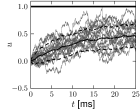
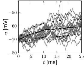
In proximity to the firing threshold the above arguments break down; however, in the subthreshold regime the mean and the variance of the membrane potential are well approximated by formulas (8.11) and (8.13), respectively. The mean trajectory and the standard deviation of the fluctuations can also be estimated in simulations, as shown in Fig. 8.3 for the leaky and the exponential integrate-and-fire models.

Fig. 8.3: Mean trajectory and fluctuations for (A) the leaky integrate-and-fire model and (B) the exponential integrate-and-fire model driven by white noise superimposed on a constant input that drives the neuron half-way between resting potential and firing threshold. Integration starts at $u=u_{r}$ and is repeated for 15 trials (gray lines). Thick line indicates mean trajectories and dashed lines indicate one standard deviation around the mean. Both models have a time constant of $10$ ms. The threshold is at $1$ for the leaky integrate-and-fire neuron (A) and at $-50$ mV for the exponential integrate-and-fire neuron (B). The numerical threshold is set at $\theta_{\rm reset}=-30$ mV.

8.1.3 Colored Noise

A noise term with a power spectrum which is not flat is called colored noise. Colored noise $I^{\rm noise}(t)$ can be generated from white noise by suitable filtering. For example, low-pass filtering

\tau_{s}{{\text{d}}I^{\rm noise}(t)\over{\text{d}}t}=-I^{\rm noise}(t)+\xi(t),

(8.15)

where $\xi(t)$ is the white noise process defined above, yields colored noise with reduced power at frequencies above $1/\tau_{s}$ . Eq. (8.15) is another example of an Ornstein-Uhlenbeck process.

In order to calculate the power spectrum of the colored noise defined in Eq. (8.15), we proceed in two steps. First we integrate (8.15) so as to arrive at

I^{\rm noise}(t)=\int_{0}^{\infty}\kappa(s)\,\xi(t-s)\,{\text{d}}s,

(8.16)

where $\kappa(s)$ is an exponential low-pass filter with time constant $\tau_{s}$ . The autocorrelation function is therefore

\langle I^{\rm noise}(t)I^{\rm noise}(t^{\prime})\rangle=\int_{0}^{\infty}\int% _{0}^{\infty}\kappa(s)\,\kappa(s^{\prime})\,\langle\xi(t-s)\,\xi(t^{\prime}-s^% {\prime})\rangle\,\,{\text{d}}s^{\prime}{\text{d}}s.

(8.17)

Second, we exploit the definition of the white noise correlation function in (8.4), and find

\langle I^{\rm noise}(t)I^{\rm noise}(t^{\prime})\rangle=a\,\exp(-{|t-t^{% \prime}|\over\tau_{s}})

(8.18)

with an amplitude factor $a$ . Therefore, knowledge of the input current at time $t$ gives us a hint about the input current shortly afterward, as long as $|t^{\prime}-t|\ll\tau_{s}$ .

The noise spectrum is the Fourier transform of (8.18). It is flat for frequencies $\omega\ll 1/\tau_{s}$ and falls off for $\omega>1/\tau_{s}$ . Sometimes, $1/\tau_{s}$ is called the cut-off frequency.

The colored noise defined in (8.15) is a suitable noise model for synaptic input, if spikes arrive stochastically and synapses have a finite time constant $\tau_{s}$ . The relation of input noise to stochastic spike arrival is the topic of the next section.