1.4 Limitations of the Leaky Integrate-and-Fire Model
The leaky integrate-and-fire model presented in Section 1.3 is highly simplified and neglects many aspects of neuronal dynamics. In particular, input, which may arise from presynaptic neurons or from current injection, is integrated linearly, independently of the state of the postsynaptic neuron:
| (1.31) |
where is the input current. Furthermore, after each output spike the membrane potential is reset,
| (1.32) |
so that no memory of previous spikes is kept. Let us list the major limitations of the simplified model discussed so far. All of these limitations will be addressed in the extension of the leaky integrate-and-fire model presented in Part II of the book.
1.4.1 Adaptation, Bursting, and Inhibitory Rebound
To study neuronal dynamics experimentally, neurons can be isolated and stimulated by current injection through an intracellular electrode. In a standard experimental protocol we could, for example, impose a stimulating current that is switched at time from a value to a new value . Let us suppose that so that the neuron is quiescent for . If the current is sufficiently large, it will evoke spikes for . Most neurons will respond to the current step with a spike train where intervals between spikes increase successively until a steady state of periodic firing is reached; cf. Fig. 1.10C. Neurons that show this type of adaptation are called regularly-firing neurons (102). Adaptation is a slow process that builds up over several spikes. Since the standard leaky integrate-and-fire model resets the voltage after each spike to the same value and restarts the integration process, no memory is kept beyond the most recent spike. Therefore, the leaky integrate-and-fire neuron cannot capture adaptation. Detailed neuron models, which will be discussed in Chapter 2, explicitly describe the slow processes that lead to adaptation. To mimic these processes in integrate-and-fire neurons, we need to add up the contributions to refractoriness of several spikes back in the past. As we will see in Chapter 6, this can be done in the ‘filter’ framework of Eq. (1.22) by using a filter for refractoriness with a time constant much slower than that of the membrane potential. Or by combining the differential equation of the leaky integrate-and-fire model with a second differential equation describing the evolution of a slow variable; cf. Chapter 6.
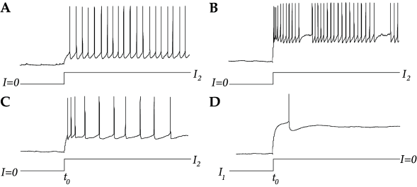
A second class of neurons are fast-spiking neurons. These neurons show no adaptation (cf. Fig. 1.10A) and can therefore be well approximated by non-adapting integrate-and-fire models. Many inhibitory neurons are fast-spiking neurons. Apart from regular-spiking and fast-spiking neurons, there are also bursting and stuttering neurons which form a separate group (102). These neurons respond to constant stimulation by a sequence of spikes that is periodically (bursting) or aperiodically (stuttering) interrupted by rather long intervals; cf. Fig. 1.10B. Again, a neuron model that has no memory beyond the most recent spike cannot describe bursting, but the framework in Eq. (1.22) with arbitrary ‘filters’ is general enough to account for bursting as well.
Another frequently observed behavior is post-inhibitory rebound. Consider a step current with and , i.e., an inhibitory input that is switched off at time ; cf. Fig. 1.10D. Many neurons respond to such a change with one or more ‘rebound spikes’: Even the release of inhibition can trigger action potentials. We will return to inhibitory rebound in Chapter 3.
1.4.2 Shunting Inhibition and Reversal Potential
In the previous paragraph we focused on an isolated neuron stimulated by an applied current. In reality, neurons are embedded into a large network and receive input from many other neurons. Suppose a spike from a presynaptic neuron is sent at time towards the synapse of a postsynaptic neuron . When we introduced in Fig. 1.5 the postsynaptic potential that is generated after the arrival of the spike at the synapse, its shape and amplitude did not depend on the state of the postsynaptic neuron . This is of course a simplification and reality is somewhat more complicated. In Chapter 3 we will discuss detailed neuron models that describe synaptic input as a change of the membrane conductance. Here we simply summarize the major phenomena.
In Fig. 1.11 we have sketched schematically an experiment where the neuron is driven by a constant current . We assume that is too weak to evoke firing so that, after some relaxation time, the membrane potential settles at a constant value . At one of the presynaptic neurons emits a spike so that shortly afterwards the action potential arrives at the synapse and provides additional stimulation of the postsynaptic neuron. More precisely, the spike generates a current pulse at the postsynaptic neuron (postsynaptic current, PSC) with amplitude
| (1.33) |
where is the membrane potential and is the ‘reversal potential’ of the synapse. Since the amplitude of the current input depends on , the response of the postsynaptic potential does so as well. Reversal potentials are systematically introduced in Chapter 2; models of synaptic input are discussed in Chapter 3.1.
Example: Shunting inhibition
The dependence of the postsynaptic response upon the momentary state of the neuron is most pronounced for inhibitory synapses. The reversal potential of inhibitory synapses is below, but usually close to the resting potential. Input spikes thus have hardly any effect on the membrane potential if the neuron is at rest; cf. Fig. 1.11A. However, if the membrane is depolarized, the very same input spikes evoke a larger inhibitory postsynaptic potential. If the membrane is already hyperpolarized, the input spike can even produce a depolarizing effect. There is an intermediate value – the reversal potential – where the response to inhibitory input ‘reverses’ from hyperpolarizing to depolarizing.
Though inhibitory input usually has only a small impact on the membrane potential, the local conductivity of the cell membrane can be significantly increased. Inhibitory synapses are often located on the soma or on the shaft of the dendritic tree. Due to their strategic position, a few inhibitory input spikes can ‘shunt’ the whole input that is gathered by the dendritic tree from hundreds of excitatory synapses. This phenomenon is called ‘shunting inhibition’.
The reversal potential for excitatory synapses is usually significantly above the resting potential. If the membrane is depolarized the amplitude of an excitatory postsynaptic potential is reduced, but the effect is not as pronounced as for inhibition. For very high levels of depolarization a saturation of the EPSPs can be observed; cf. 1.11B.
| A | B |
|---|---|

|
 |
1.4.3 Conductance Changes after a Spike
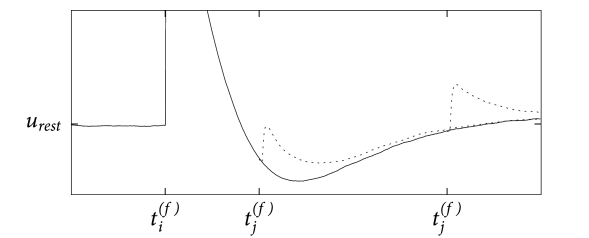
The shape of the postsynaptic potentials does not only depend on the level of depolarization but, more generally, on the internal state of the neuron, e.g., on the timing relative to previous action potentials.
Suppose that an action potential has occurred at time and that a presynaptic spike arrives at a time at the synapse . The form of the postsynaptic potential depends now on the time ; cf. Fig. 1.12. If the presynaptic spike arrives during or shortly after a postsynaptic action potential, it has little effect because some of the ion channels that were involved in firing the action potential are still open. If the input spike arrives much later, it generates a postsynaptic potential of the usual size. We will return to this effect in Chapter 2.
1.4.4 Spatial Structure
The form of postsynaptic potentials also depends on the location of the synapse on the dendritic tree. Synapses that are located far away from the soma are expected to evoke a smaller postsynaptic response at the soma than a synapse that is located directly on the soma; cf. Chapter 3. If several inputs occur on the same dendritic branch within a few milliseconds, the first input will cause local changes of the membrane potential that influence the amplitude of the response to the input spikes that arrive slightly later. This may lead to saturation or, in the case of so-called ‘active’ currents, to an enhancement of the response. Such nonlinear interactions between different presynaptic spikes are neglected in the leaky integrate-and-fire model. Whereas a purely linear dendrite can be incorporated in the ‘filter’ description of the model, as we will see in Chapter 6, nonlinear interactions cannot. Small regions on the dendrite where a strong nonlinear boosting of synaptic currents occurs are sometimes called dendritic ’hot spots’. The boosting can lead to dendritic spikes which, in contrast to normal somatic action potentials last for tens of milliseconds (289).