10.3 Evaluating Goodness-of-fit
No single method provides a complete assessment of goodness-of-fit; rather, model fitting should always be seen as a loop, in which we start by fitting a model, then examine the results, attempt to diagnose any model failures, and then improve our models accordingly. In the following, we describe different methods for assessing the goodness-of-fit.
Before beginning with specific examples of these methods, we note that it is very important to evaluate the goodness of fit on data that was not used for fitting. The part of the data used for fitting model parameters is called the training set and the part of the data reserved to evaluate the goodness of fit is called the test set. Data in the test set is said to be predicted by the model, while it is simply reproduced in the training set. By simply adding parameters to the model, the quality of the fit on the training set increases. Given a sufficient number of parameters, the model might be able to reproduce the training set perfectly, but that does not mean that data in the test set is well predicted. In fact it is usually the opposite: overly complicated models that are ‘overfit’ on the training data (i.e., which fit not only the reproducible signal in the training set but also the noise) will often do a bad job generalizing and predicting new data in the test set. Thus in the following we assume that the goodness of fit quantities are computed using ‘cross-validation’: parameters are estimated using the training set, and then the goodness of fit quantification is performed on the test set.
10.3.1 Comparing Spiking Membrane Potential Recordings
Given a spiking membrane potential recording, we can use traditional measures such as the squared error between model and recorded voltage to evaluate the goodness of fit. This approach, however, implicitly assumes that the remaining error has a Gaussian distribution (recall the close relationship between Gaussian noise and the squared error, discussed above). Under diffusive noise, we have seen (Chapter 8) that membrane potential distributions are Gaussian only when all trajectories started at the same point and none have reached threshold. Also, a small jitter in the firing time of the action potential implies a large error in the membrane potential, much larger than the typical subthreshold membrane potential variations. For these two reasons, the goodness-of-fit in terms of subthreshold membrane potential away from spikes is considered separately from the goodness-of-fit in terms of the spike times only.
In order to evaluate how the model predicts subthreshold membrane potential we must compare the average error with the intrinsic variability. To estimate the first of these two quantities, we compute the squared error between the recorded membrane potential and model membrane potential with forced spikes at the times of the observed ones. Since spike times in the model are made synchronous with the experimental recordings, all voltage traces start at the same point. A Gaussian assumption thus justified, we can average the squared error over all recorded times that are not too close to an action potential:
| (10.37) |
where refers to the ensemble of time bins at least 5 ms before or after any spikes and is the total number of time bins in . has index for ‘neuron’ and index for ‘model’. It estimates the error between the real neuron and the model.
To evaluate the second quantity, we compare recorded membrane potential from multiple repeated stimulations having the same stimulus. Despite the variability in spike timings, it is usually possible to find times which are sufficiently away from a spike in any repetition and compute the averaged squared error
| (10.38) |
where refers to the ensemble of time bins far from the spike times in any repetition and is the total number of time bins in . Typically, 20 ms before and 200 ms after the spike is considered sufficiently far. Note that with this approach we implicitly assume that spike-afterpotentials have vanished 200ms after a spike. However, as we will see in Chapter 11, the spike afterpotentials can extend for more than one second, so that the above assumption is a rather bad approximation. Because the earlier spiking history will affect the membrane potential, the RMSE calculated in Eq. (10.38) is an overestimate.
To quantify the predictive power of the model, we finally compute the model error with the intrinsic error by taking the ratio
| (10.39) |
The root-mean-squared-error ratio (RMSER) reaches one if the model precision is matched with intrinsic error. When smaller than one, the RMSER indicates that the model could be improved. Values larger than one are possible because RMSE is an overestimate of the true intrinsic error.
10.3.2 Spike Train Likelihood
The likelihood is the probability of generating the observed set of spike times with the current set of parameters in our stochastic neuron model. It was defined in Eq. (9.10) of Sect. 9.2 which we reproduce here
| (10.40) |
where we used to emphasize that the firing intensity of a spike at depends on both the stimulus and spike history as well as the model parameters .
The likelihood is a conditional probability density and has units of inverse time to the power of (where is the number of observed spikes). To arrive at a more interpretable measure, it is common to compare with the likelihood of a homogeneous Poisson model with a constant firing intensity , i.e., a Poisson process which is expected to generate the same number of spikes in the observation interval . The difference in log-likelihood between the Poisson model and the neuron model is finally divided by the total number of observed spikes in order to obtain a quantity with units of ‘bits per spike’:
| (10.41) |
This quantity can be interpreted as an instantaneous mutual information between the spike count in a single time bin and the stimulus given the parameters. Hence, it is interpreted as a gain in predictability produced by the set of model parameters . One advantage of using the log-likelihood of the conditional firing intensity is that it does not require multiple stimulus repetitions. It is especially useful to compare on a given data set the performances of different models: better models achieve higher cross-validated likelihood scores.
10.3.3 Time-rescaling Theorem
For a spike train with spikes at and with firing intensity , the time-rescaling transformation is defined as
| (10.42) |
It is a useful and somewhat surprising result that (evaluated at the measured firing times) is a Poisson process with unit rate (73). A correlate of this time-rescaling theorem is that the time intervals
| (10.43) |
are independent random variables with an exponential distribution (c.f. Chapter 7). Re-scaling again the time axis with the transformation
| (10.44) |
forms independent uniform random variables on the interval zero to one.
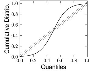
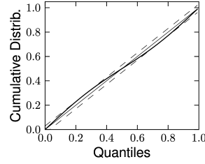
Therefore, if the model is a valid description of the spike train , then the resulting should have the statistics of a sequence of independent uniformly distributed random variables. As a first step, one can verify that the ’s are independent by looking at the serial correlation of the interspike intervals or by using a scatter plot of against . Testing whether the ’s are uniformly distributed can be done with a Kolmogorov-Smirnov (K-S) test. The K-S statistic evaluates the distance between the empirical cumulative distribution function of , , and the cumulative distribution of the reference function. In our case, the reference function is the uniform distribution, so that its cumulative is simply . Thus,
| (10.45) |
The K-S statistic converges to zero as the empirical probability converges to the reference. The K-S test then compares with the critical values of the Kolmogorov distribution. Figure 10.6 illustrates two examples: one where the empirical distribution was far from a uniform distribution and the other where the model rescaled time correctly. See (173) for a multivariate version of this idea that is applicable to the case of coupled neurons. To summarize, the time-rescaling theorem along with the K-S test provide a useful goodness-of-fit measure for spike train data with confidence intervals that does not require multiple repetitions.
| A | B |
|---|---|
|
 |
10.3.4 Spike Train Metric
Evaluating the goodness-of-fit in terms of log-likelihood or the time-rescaling theorem requires that we know the conditional firing intensity accurately. For biophysical models as seen in Chapter 2 but complemented with a source of variability, the firing intensity is unavailable analytically. The intensity can be estimated numerically by simulating the model with different realizations of noise, or by solving a Fokker-Planck equation, but this is sometimes impractical.
Another approach for comparing spike trains involves defining a metric between spike trains. Multiple spike timing metrics have been proposed, with different interpretations. A popular metric was proposed by Victor and Purpura (1996). Here, we describe an alternative framework for the comparison of spike trains that makes use of vector space ideas, rather than more general metric spaces.
| A | B |
|---|---|
 |
|
Let us consider spike trains as vectors in an abstract vector space, with these vectors denoted with boldface: . A vector space is said to have an inner (or scalar) product if for each vector pair and there exists a unique real number satisfying the following axioms: commutativity, distributivity, associativity and positivity. There are multiple candidate inner products satisfying the above axioms. The choice of inner product will be related to the type of metric being considered. For now, consider the general form
| (10.46) |
where is a two-dimensional coincidence kernel with a scaling parameter , and is the maximum length of the spike trains. is required to be a non-negative function with a global maximum at . Moreover, should fall off rapidly so that for all . Examples of kernels include . For instance, is a kernel that was used by van Rossum (531). The scaling parameter must be small, much smaller than the length of the spike train.
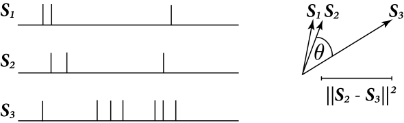
For a comparison of spike-trains seen as vectors the notions of angular separation, distance and norm of spike trains are particularly important. The squared norm of a spike train will be written . With , we observe that where is the number of spikes in . Therefore the norm of a spike train is related to the total number of spikes it contains. The Victor and Purpura metric is of a different form than the form discussed here, but it has similar properties (see exercies).
The norm readily defines a distance, , between two spike-trains
| (10.47) |
The right hand side of Eq. (10.47) shows that that the distance between two spike trains is maximum when is zero. On the other hand, becomes zero only when . This implies that . Again consider , then is the total number of spikes in both and reduced by 2 for each spike in that coincided with one in . For the following, it is useful to think of a distance between spike trains as a number of non-coincident spikes.
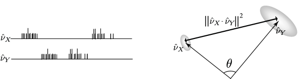
The cosine of the angle between and is
| (10.48) |
This angular separation relates to the fraction of coincident spikes. Fig. 10.7 illustrate the concepts of angle and distance for spike trains seen as vectors.
| A | B |
|---|---|
 |
|
10.3.5 Comparing Sets of Spike Trains
Metrics such as described above can quantify the similarity between two spike trains. In the presence of variability, however, a simple comparison of spike trains is not sufficient. Instead, the spike train similarity measure must be maximally sensitive to differences in the underlying stochastic processes.
We want to know if spike trains generated from a neuron model could well have been generated by a real neuron. We could simply calculate the distance between a spike train from the neuron and a spike train from the model, but neurons are noisy and we will find a different distance each time we repeat the recording. To achieve better statistics, we can compare a set of spike trains from the model with a set of spike trains from the neuron.
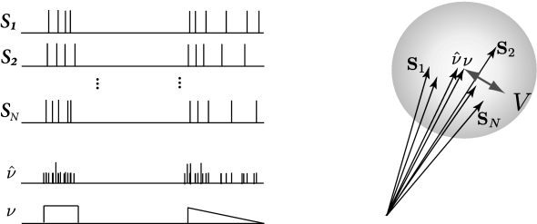
Let the two sets of spike trains be denoted by and , containing and spike trains, respectively. First, it is useful to define some characteristics of such sets of spike trains. A natural quantity to consider is the average of the norms of each spike train within a set, say ,
| (10.49) |
where we have used ‘’ to denote that the quantity is an experimental estimate. We note that is related to the averaged spike count. is exactly the averaged spike count if the inner product satisfies i) and ii) whenever is greater than the minimum interspike interval of any of the spike trains considered. The interpretation spike count is helpful for the discussion in the remainder of this section. Furthermore, the vector of averaged spike trains
| (10.50) |
is another occurrence of the spike density seen in Chapter 7. It defines the instantaneous firing rate of the the spiking process, .
| A | B |
|---|---|
 |
|
In the vector space, can be thought of as lying at the center of the spike trains seen as vectors (Fig. 10.9), note that other ‘mean spike train’ could be defined (561). The size of the cloud quantifies the variability in the spike timing. The variability is defined as the variance
| (10.51) |
A set of spike trains where spikes always occur at the same times has low variability. When the spikes occur with some jitter around a given time, the variability is larger. Variability relates to reliability. While variability is a positive quantity that can not exceed , reliability is usually defined between zero and one where one means perfectly reliable spike timing: .
Finally, we come to a measure of match between the set of spike trains and . The discussion in Chapter 7 about the neural code would suggest that neuron models should reproduce the detailed time structure of the PSTH. We there define
| (10.52) |
We have (for match) equal to one if and have the same instantaneous firing rate. The smaller the greater the mismatch between the spiking processes. The quantity can be interpreted as a number of reliable spikes. Since is interpreted as a number of coincident spikes between and , we can still regard as a factor counting the fraction of coincident spikes. A similar quantity can be defined for metrics that can not be cast into a inner product (357).
If the kernel is chosen to be and is a Gaussian distribution of width , then relates to a mean square error between PSTHs that were filtered with . Therefore, the kernel used in the definition of the inner product (Eq. (10.46)) can be related to the smoothing filter of the PSTH (see Exercises).