10.2 Statistical Formulation of Encoding Models
Let us denote the observed spike train data by . In general, could represent measurements from a population of neurons. To keep the arguments simple, we focus for the moment on a single neuron, but at the end of the section we will extend the approach to a population of interacting neurons. If the time bins are chosen smaller than the absolute refractory period, the discretized spike train is described by a sequence of scalar variables in an interval
| (10.15) |
cf. Fig. 9.6 in Chapter 9. If time bins are large, spike counts can take values larger than one.
A neural ‘encoding model’ is a model that assigns a conditional probability, , to any possible neural response given a stimulus . The vector can include the momentary stimulus presented at time , or more generally the concatenated spatiotemporal stimulus history up to time . Examples have been given in Section 10.1.
As emphasized in the introduction to this chapter, it is not feasible to directly measure this probability for all stimulus-response pairs , simply because there are infinitely many potential stimuli. We therefore hypothesize some encoding model,
| (10.16) |
Here is a short-hand notation for the set of all model parameters. In the examples of the previous section, the model parameters are .
Our aim is to estimate the model parameters so that the model ‘fits’ the observed data . Once is in hand we may compute the desired response probabilities as
| (10.17) |
that is, knowing allows us to interpolate between the observed (noisy) stimulus-response pairs, in order to predict the response probabilities for novel stimuli for which we have not yet observed any responses.
10.2.1 Parameter estimation
How do we find a good estimate for the parameters for a chosen model class? The general recipe is as follows. The first step is to introduce a model that makes sense biophysically, and incorporates our prior knowledge in a tractable manner. Next we write down the likelihood of the observed data given the model parameters, along with a prior distribution that encodes our prior beliefs about the model parameters. Finally, we compute the posterior distribution of the model parameters given the observed data, using Bayes’ rule, which states that
| (10.18) |
the left-hand side is the desired posterior distribution, while the right-hand side is just the product of the likelihood and the prior.
In the current setting, we need to write down the likelihood of the observed spike data given the model parameter and the observed set of stimuli summarized in the matrix , and then we may employ standard likelihood optimization methods to obtain the maximum likelihood (ML) or maximum a posteriori (MAP) solutions for , defined by
| (10.19) | |||||
| (10.20) |
where the maximization runs over all possible parameter choices.
We assume that spike counts per bin follow a conditional Poisson distribution, given :
| (10.21) |
cf. text and exercises of Chapter 7. For example, with the rate parameter of the Poisson distribution given by a GLM or SRM model , we have
| (10.22) |
Here denotes the product over all time steps. We recall that, by definition, for .
Our aim is to optimize the parameter . For a given observed spike train, the spike count numbers are fixed. In this case, is a constant which is irrelevant for the parameter optimization. If we work with a fixed time step and drop all units, we can therefore reshuffle the terms and consider the logarithm of the above likelihood
| (10.23) |
If we choose the time step shorter than the half-width of an action potential, say 1 ms, the spike count variable can only take the values zero or one. For small , the likelihood of Eq. (10.22) is then identical to that of the SRM with escape noise, defined in Chapter 9; cf. Eqs. (9.10) and (9.15) - (9.17).
We don’t have an analytical expression for the maximum of the likelihood defined in Eq. (10.22), but nonetheless we can numerically optimize this function quite easily if we are willing to make two assumptions about the nonlinear function . More precisely, if we assume that
(i) is a convex (upward-curving) function of its scalar argument , and
(ii) is concave (downward-curving) in ,
then the loglikelihood above is guaranteed to be a concave function of the parameter , since in this case the loglikelihood is just a sum of concave functions of (383).
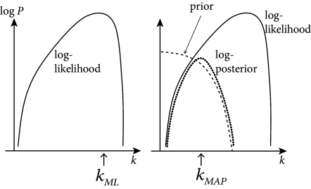
This implies that the likelihood has no non-global maximum (also called local maximum). Therefore the maximum likelihood parameter may be found by numerical ascent techniques; cf. Fig. 10.2. Functions satisfying these two constraints are easy to think of: for example, the standard linear rectifier and the exponential function both work.
Fitting model parameters proceeds as follows: we form the (augmented) matrix where each row is now
| (10.24) |
Similarly, the parameter vector is in analogy to Eq. (10.10)
| (10.25) |
here is a constant offset term which we want to optimize.
We then calculate the log-likelihood
| (10.26) |
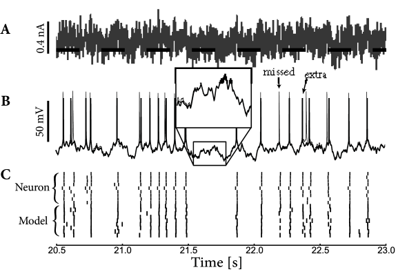
and compute the ML or maximum a posteriori (MAP) solution for the model parameters by a concave optimization algorithm. Note that, while we still assume that the conditional spike count within a given short time bin is drawn from a one-dimensional distribution given , the resulting model displays strong history effects (since depends on the past spike trains) and therefore the output of the model, considered as a vector of counts , is no longer a Poisson process, unless . Importantly, because of the refractory effects incorporated by a strong negative at small times, the spike count variable cannot take a value larger than if is in the range of one or a few milliseconds. Therefore, we can expect that interspike intervals are correctly reproduced in the model; see Fig. 10.5 for an example application.
Finally, we may expand the definition of to include observations of other spike trains, and therefore develop GLMs not just of single spike trains, but network models of how populations of neurons encode information jointly (95; 379; 521; 399). The resulting model is summarized as follows: Spike counts are conditionally Poisson distributed given with a firing rate
| (10.27) |
Here, denotes the instantaneous firing rate of the -th cell at time and is the cell’s linear receptive field including spike-history effects; cf. Eq. (10.25). The net effect of a spike of neuron onto the membrane potential of neuron is summarized by ; these terms are summed over all past spike activity in the population of cells from which we are recording simultaneously. In the special case that we record from all neurons in the population, can be interpreted as the excitatory or inhibitory postsynaptic potential caused by a spike of neuron a time earlier.
Example: Linear regression and voltage estimation
It may be helpful to draw an analogy to linear regression here. We want to show that the standard procedure of least-square minimization can be linked to statistical parameter estimation under the assumption of Gaussian noise.
We consider the linear voltage model of Eq. (10.1). We are interested in the temporal filter properties of the neuron when it is driven by a time-dependent input . Let us set and . If we assume that the discrete-time voltage measurements have a Gaussian distribution around the mean predicted by the model of Eq. (10.4), then we need to maximize the likelihood
| (10.28) |
where is the matrix of observed stimuli, are constants that do not depend on the parameter , and the sum in is over all observed time bins. Maximization yields which determines the time course of the filter that characterizes the passive membrane properties. The result is identical to Eq. (10.8):
| (10.29) |
10.2.2 Regularization: maximum penalized likelihood
In the linear regression case it is well-known that estimates of the components of the parameter vector can be quite noisy when the dimension of is large. The noisiness of the estimate is roughly proportional to the dimensionality of (the number of parameters in that we need to estimate from data) divided by the total number of observed samples (382). The same ‘overfitting’ phenomenon (estimator variability increasing with number of parameters) occurs in the GLM context. A variety of methods have been introduced to ‘regularize’ the estimated , to incorporate prior knowledge about the shape and/or magnitude of the true to reduce the noise in . One basic idea is to restrict to lie within a lower-dimensional subspace; we then employ the same fitting procedure to estimate the coefficients of within this lower-dimensional basis (model selection procedures may be employed to choose the dimensionality of this subspace (521)).
A slightly less restrictive approach is to maximize the posterior
| (10.30) |
(with allowed to take values in the full original basis), instead of the likelihood ; here encodes our a priori beliefs about the true underlying .
It is easy to incorporate this maxima a posteriori idea in the GLM context (383): we simply maximize
| (10.31) | |||||
| (10.32) |
Whenever is a concave function of , this ‘penalized’ likelihood (where acts to penalize improbable values of ) is a concave function of , and ascent-based maximization may proceed (with no local maximum) as before; cf. Fig. 10.4.
Example: Linear regression and Gaussian prior
In the linear regression case, the computationally-simplest prior is a zero-mean Gaussian, , where is a positive definite matrix (the inverse covariance matrix). The Gaussian prior can be combined with the Gaussian noise model of Eq. (10.28). Maximizing the corresponding posterior analytically (452; 485) leads then directly to the regularized least-square estimator
| (10.33) |
10.2.3 Fitting Generalized Integrate-and-Fire models to Data
Suppose an experimentalist has injected a time-dependent current into a neuron and has recorded with a second electrode the voltage of the same neuron. The voltage trajectory contains spikes with firing times . The natural approach would be to write down the joint likelihood of observing both the spike times and the subthreshold membrane potential (381). A simpler approach would be to maximize the likelihood of observing the spike separately from the likelihood of observing the membrane potential.
Given the input and the spike train , the voltage of a SRM is given by Eq. (10.9) and we can adjust the parameters of the filter and so as to minimize the squared error Eq. (10.5). We now fix the parameters for the membrane potential and maximize the likelihood of observing the spike times given our model voltage trajectory . We insert into the escape rate function which contains the parameters of the threshold
| (10.34) |
We then calculate the log-likelihood
| (10.35) |
and compute the ML or maximum a posteriori (MAP) solution for the model parameters (which are the parameters of the threshold - the subthreshold voltage parameters are already fixed) by an optimization algorithm for concave functions.
Fig. 10.5 shows an example application. Both voltage in the subthreshold regime and spike times are nicely reproduced. Therefore, we can expect that interspike intervals are correctly reproduced as well. In order to quantify the performance of neuron models, we need the develop criteria of ‘goodness of fit’ for subthreshold membrane potential, spike timings, and possibly higher-order spike train statistics. This is the topic of section 10.3; we will return to similar applications in the next chapter.
10.2.4 Extensions (*)
The GLM encoding framework described here can be extended in a number of important directions. We briefly describe two such directions here.
First, as we have described the GLM above, it may appear that the model is restricted to including only linear dependencies on the stimulus , through the term. However, if we modify our input matrix once again, to include nonlinear transformations of the stimulus , we may fit nonlinear models of the form
| (10.36) |
efficiently by maximizing the loglikelihood with respect to the weight parameter (560; 12). Mathematically, the nonlinearities may take essentially arbitrary form; physiologically speaking, it is clearly wise to choose to reflect known facts about the anatomy and physiology of the system (e.g., might model inputs from a presynaptic layer whose responses are better-characterized than are those of the neuron of interest (450)).
Second, in many cases it is reasonable to include terms in that we may not be able to observe or calculate directly (e.g., intracellular noise, or the dynamical state of the network); fitting the model parameters in this case requires that we properly account for these ‘latent,’ unobserved variables in our likelihood. While inference in the presence of these hidden parameters is beyond the scope of this chapter, it is worth noting that this type of model may be fit tractably using generalizations of the methods described here, at the cost of increased computational complexity, but the benefit of enhanced model flexibility and realism (484; 563; 536).
Example: Estimating spike triggered currents and dynamic threshold
In Fig. 10.1A, we have suggested to estimate the filter by extracting its values at discrete equally spaced time steps: The integral is linear in the parameters.
However, the observables remain linear in the parameters () if we set with fixed time constants, e.g., ms. Again, the integral is linear in the parameters. The exponentials play the role of ‘basis functions’ .
Similarly, the threshold filter or the spike-afterpotential can be expressed with basis functions. A common choice is to take rectangular basis functions which take a value of unity on a finite interval . Exponential spacing ms of time points allows us to cover a large time span with a small number of parameters. Regular spacing leads back to the naive discretization scheme.