9.2 Likelihood of a spike train | Neuronal Dynamics online book

In the previous subsection, we calculated the probability of firing in a short time step $\Delta t$ from the continuous-time firing intensity $\rho(t)$ . Here we ask a similar question, but not on the level of a single spike, but on that of a full spike train.

Suppose we know that a spike train has been generated by an escape noise process

\rho(t)=f(u(t)-\vartheta)

(9.9)

as in Eq. (9.2), where the membrane potential $u(t)$ arises from the dynamics of one of the generalized integrate-and-fire models such as the SRM.

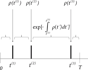
The likelihood $L^{n}$ that spikes occur at the times $t^{(1)},\dots,t^{(f)},\dots,t^{(n)}$ is (69)

\displaystyle L^{n}(\{t^{(1)},t^{(2)},\dots,t^{(n)}\})=\rho(t^{(1)})\cdot\rho(% t^{(2)})\cdot\,\dots\rho(t^{(n)})\,\exp[-\int_{0}^{T}\rho(s){\text{d}}s]\,,

(9.10)

where $[0,T]$ is the observation interval. The product on the right-hand side contains the momentary firing intensity $\rho(t^{(f)})$ at the firing times $t^{(1)},t^{(2)},\dots,t^{(n)}$ . The exponential factor takes into account that the neuron needs to ‘survive’ without firing in the intervals between the spikes.

In order to highlight this interpretation it is convenient to take a look at Fig. 9.6A and rewrite Eq. (9.10) in the equivalent form

$\displaystyle L^{n}(\{t^{(1)},t^{(2)},\dots,t^{(n)}\})=$		$\displaystyle\exp[-\int_{0}^{t^{(1)}}\rho(s){\text{d}}s]\cdot$	(9.11)
	$\displaystyle\rho(t^{(1)})$	$\displaystyle\exp[-\int_{t^{(1)}}^{t^{(2)}}\rho(s){\text{d}}s]\cdot$
	$\displaystyle\rho(t^{(2)})$	$\displaystyle\exp[-\int_{t^{(2)}}^{t^{(3)}}\rho(s){\text{d}}s]\cdot\,\dots$
	$\displaystyle\rho(t^{(n)})$	$\displaystyle\exp[-\int_{t^{(n)}}^{T}\rho(s){\text{d}}s]\,.$

Intuitively speaking, the likelihood of finding $n$ spikes at times $t^{(f)}$ depends on the instantaneous rate at the time of the spikes and the probability to survive the intervals in between without firing; cf. the survivor function introduced in Chapter 7, Eq. (7.26).

Instead of the likelihood, it is sometimes more convenient to work with the logarithm of the likelihood, called the log-likelihood

\displaystyle{\rm log}L^{n}(\{t^{(1)},\dots,t_{i}^{(f)},\dots,t^{(n)}\})=-\int% _{0}^{T}\rho(s){\text{d}}s+\sum_{f=1}^{n}{\rm log}\rho(t_{i}^{(f)}).

(9.12)

The three formulations Eqs. (9.10) – (9.12) are equivalent and it is a matter of taste if one is preferred over the others.

Example: Discrete-time version of likelihood and generative model

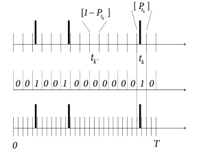
In a discrete-time simulation of a SRM or generalized integrate-and-fire model with escape noise, we divide the simulation interval $[0,T]$ into $N$ time steps $\Delta t=T/N$ ; cf. Fig. 9.6B. In each time step, we first calculate the membrane potential $u(t)$ and then generate a spike with probability $P_{t}=P_{F}(u(t))$ given by Eq. (9.8). To do so, we call on the computer a random number $r_{t}$ between zero and unity. If $P_{t}>r_{t}$ , a spike is generated, i.e., the spike count number in this time bin is $n_{t}=1$ . The probability of finding an empty time bin (spike count $n_{t}=0$ ) is

{\rm Prob}\left\{{\rm silent~{}in~{}}[t,t+\Delta t]\right\}=1-P_{t}=\exp\left% \{-\Delta t\,\rho(t)\right\}\,

(9.13)

where we have assumed that time bins are short enough so that the membrane potential does not change a lot from one time step to the next. The spike train can be summarized as sequence $\{0,0,1,0,0,0,1,0,\dots\}$ of $N$ binary numbers $n_{t}\in\{0,1\}$ . We emphasize that, with the above discrete-time spike generation model it is impossible to have two spikes in a time bin $\Delta t$ . This reflects the fact that, because of neuronal refractoriness, neurons cannot emit two spikes in a time bin shorter than, say, half the duration of an action potential.

Since we call an independent random number in each time bin, a specific spike train occurs with a probability given by the product of the probabilities per bin:

	$\displaystyle P_{\rm total}$	$\displaystyle=$	$\displaystyle\Pi_{bins~{}with~{}spike}[P_{t}]\,\cdot\,\Pi_{empty~{}bins}[1-P_{% t}]$		(9.14)
		$\displaystyle=$	$\displaystyle\Pi_{t}\left\{[P_{t}]^{n_{t}}\,\cdot\,[1-P_{t}]^{1-n_{t}}\right\},$		(9.15)

where the product runs over all time bins and $n_{t}\in\{0,1\}$ is the spike count number in each bin.

We now switch our perspective and study an observed spike train in continuous time with spike firings at times $t^{(f)}$ with $0<t^{(1)},t^{(2)},\dots,t^{(n)}<T$ . The spike train was generated by a real neuron in a slice experiment under current injection with a known current $I(t)$ . We now ask the following question: What is the probability that the observed spike train could have been generated by our model? Thus, we consider our discrete-time model with escape noise as a generative model of the spike train. To do so, we calculate the voltage using a discrete-time version of Eq. (9.1). Given the (known) injected input $I(t)$ and the (observed) spike times $t^{(f)}$ , we can calculate the voltage $u(t)$ of our model and therefore the probability of firing in each time step.

The observed spike trains has $n$ spikes at times $0<t^{(1)},t^{(2)},\dots,t^{(n)}<T$ . Let us denote time bins containing a spike by $t_{k}$ with index $k$ (i.e., $t_{1}<t^{(1)}\leq t_{1}+\Delta t$ ; $t_{2}<t^{(2)}\leq t_{2}+\Delta t;\dots$ ) and empty bins by $t_{k^{\prime}}$ with a dummy index $k^{\prime}$ . Using Eq. (9.14), the probability that the observed spike train could have been generated by our model is

\displaystyle P_{\rm total}=\Pi_{k=1}^{n}[P_{t_{k}}]\,\cdot\,\Pi_{k^{\prime},t% _{k^{\prime}}\neq t_{k}}[1-P_{t_{k^{\prime}}}]\,.

(9.16)

Eq. (9.16) is the starting point for finding optimal parameters of neuron models (Chapter 10).

We can gain some additional insights, if we rearrange the terms on the right-hand side of Eq. (9.16) differently. All time bins that fall into the interval between two spikes can be regrouped as follows

	$\displaystyle\Pi_{\{k^{\prime}\|t_{k}<t_{k^{\prime}}\leq t_{k+1}\}}[1-P_{t_{k^{% \prime}}}]$	$\displaystyle=$	$\displaystyle\Pi_{\{k^{\prime}\|t_{k}<t_{k^{\prime}}\leq t_{k+1}\}}\exp\left\{-% \Delta t\,\rho(t_{k^{\prime}})\right\}$		(9.17)
		$\displaystyle=$	$\displaystyle\exp\left\{-\sum_{t_{k}<t_{k^{\prime}}<t_{k+1}}\Delta t\,\rho(t_{% k^{\prime}})\right\}\,.$		(9.17)

Ideally, a spike train in continuous time should be described by a model in continuous time. We therefore ask whether the discretization of time is critical or whether we can get rid of it. The transition to continuous time corresponds to the limit of $N\to\infty$ while $T$ is kept fixed. The Riemann-sum on the right-hand side of Eq. (9.17) then turns into an integral. In the same limit, the contribution of the bins containing a spike to Eq. (9.16) can be written as $P_{t_{k}}=\rho(t_{k})\Delta t$ . We are led back from the discrete-time generative model to Eq. (9.11) in continuous time with the replacement

P_{\rm total}=L^{n}(\{t^{(1)},t^{(2)},\dots t^{(n)}\})(\Delta t)^{n}\,,

(9.18)

i.e., the continuum limit exists. In other words, once the time steps $\Delta t$ are short enough, the exact discretization scheme does not play a role. Alternative, more efficient, sampling schemes exist that avoid discretization (73); see Section 10.3.3 in Chapter 10.