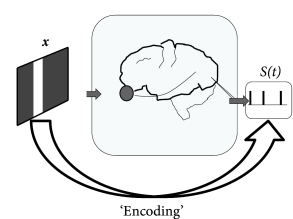
11 Encoding and Decoding with Stochastic Neuron models 11.1 Encoding Models for Intracellular Recordings 11.3 Decoding

11.2 Encoding Models in Systems Neuroscience

Generalized integrate-and-fire models have been used not only for spike prediction of neurons in brain slices, but also for measurements in systems neuroscience, i.e., in the intact brain driven by sensory stimuli or engaged in a behavioral task. Traditionally, electrophysiological measurements in vivo have been performed with extracellular electrodes or multi-electrode probes. With extracellular recording devices, the presence of spikes emitted by one or several neurons can be detected, but the membrane potential of the neuron is unknown. Therefore, in the following we aim at predicting spikes in extracellular recordings from a single neuron, or in groups of connected neurons.

Fig. 11.5: The encoding problem in visual neuroscience. A. A stimulus is presented on a screen while a spike train is recorded from an area in visual cortex. B. Models designed to predict the spike train first filter the stimulus ${\bf x}$ with a spatial filter ${\bf k}$ (linear processing step), pass the result $u={\bf k}\cdot{\bf x}$ through a nonlinearity $f$ and then generate spikes stochastically with Poisson statistics. The main difference between an Linear-Nonlinear-Poisson (LNP, top) and a soft-threshold generalized integrate-and-fire model (GLM, bottom) is the presence of spike-triggered currents $\tilde{\eta}(s)$ in the latter.

11.2.1 Receptive fields and Linear-Nonlinear Poisson Model

The linear properties of a simple neuron in primary visual cortex can be identified with its receptive field, i.e., the small region of visual space in which the neuron is responsive to stimuli (cf. Chapters 1 and 12). Receptive fields as linear filters have been analyzed in a wide variety of experimental preparations.

Experimentally, the receptive field of a simple cell in visual cortex can be determined by presenting a random sequence of spots of lights on a gray screen while the animal is watching the screen. In a very limited region of the screen, the spot of light leads to an increase in the probability of firing of the cell, in an adjacent small region to a decrease. The spatial arrangement of these regions defines the spatial receptive field of the cell and can be visualized as a two-dimensional spatial linear filter (Fig. 11.5B).

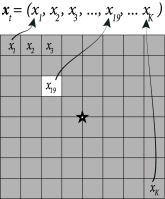
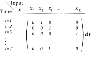
Instead of a two-dimensional notation of screen coordinates, we choose in the following a vector notation where we label all pixels with a single index $k$ . For example, on a screen with $256\times 256$ pixels we have $1\leq k\leq K$ with $K=65^{\prime}536$ . A full image corresponds to a vector $\mbox{\boldmath$x$}=(x_{1},\dots x_{K})$ while a single spot of light corresponds to a vector with all components equal to zero except one (Fig. 11.6A).

The spatial receptive field of a neuron is a vector $k$ of the same dimensionality as $x$ . The response of the neuron to an arbitrary spatial stimulus $x$ depends on the total drive $\mbox{\boldmath$k$}\cdot\mbox{\boldmath$x$}_{t}$ , i.e., the similarity between the stimulus and the spatial filter.

More generally, the receptive field filter $k$ can be described not only by a spatial component, but also by a temporal component: an input 100ms ago has less influence on the spiking probability now than an input 30ms ago. In other words, the scalar product $\mbox{\boldmath$k$}\cdot\mbox{\boldmath$x$}_{t}$ is a short-hand notation for integration over space as well as over time. Such a filter $k$ is called a spatio-temporal receptive field.

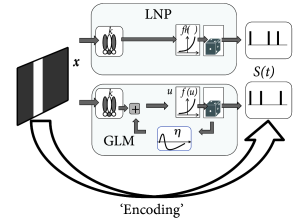
In the linear-nonlinear-Poisson (LNP) model, one assumes that spike trains are produced by an inhomogeneous Poisson process with rate

\rho(t)=f(\mbox{\boldmath\(k\)}\cdot\mbox{\boldmath\(x\)}_{t})

(11.5)

given by a cascade of two simple steps (Fig. 11.5B). The linear stage, $\mbox{\boldmath$k$}\cdot\mbox{\boldmath$x$}_{t}$ , is a linear projection of $\mbox{\boldmath$x$}_{t}$ , the (vector) stimulus at time $t$ , onto the receptive field $k$ ; this linear stage is then followed by a simple scalar nonlinearity $f(.)$ which shapes the output (and in particular enforces the non-negativity of the output firing rate $\rho(t)$ ). A great deal of the systems neuroscience literature concerns the quantification of the receptive field parameters $k$ .

Note that the LNP model neglects the spike history effects that are the hallmark of the SRM and the GLM – otherwise the two models are surprisingly similar; cf. Fig. 11.5B. Therefore, a LNP model cannot account for refractoriness or adaptation, while a GLM in the form of a generalized soft-threshold integrate-and-fire model does. The question arises whether a model with spike-history effects yields a better performance than the standard LNP model.

Fig. 11.6: Spatial receptive field measurement. A. While the animal focuses on the center (star), light dots are presented at random positions on a gray screen; in the present trial, pixel 19 lights up. The input is denoted as a vector $\mbox{\boldmath$x$}_{t}$ . B. Schematic of input matrix $X$ . Matrix representing a sparse input, such as a single spot of light. Rows of the matrix correspond to different trials, marked by the observation time $t$ .

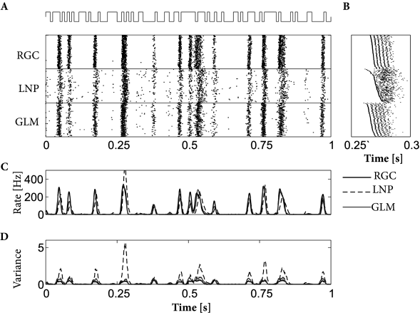
Both models, LNP and GLM, can be fitted using the methods discussed in Ch. 10. For example, the two models have been compared on a data set where retinal ganglion cells have been driven by full-field light stimulus, i.e., the stimulus did not have any spatial structure (398). Prediction performance ranged in similar values as for cortical neurons driven by intracellular current injection, with up to 90% of the PSTH variance predicted in some cases. LNP models in this context have significantly worse prediction accuracy; in particular, LNP models greatly overestimate the variance of the predicted spiking responses. See Fig. 11.7 for an example.

Example: Detour on reverse correlation for receptive field estimation

Reverse correlation measurements are an experimental procedure based on spike-triggered averaging (113; 94). Stimuli $x$ are drawn from some statistical ensemble and presented one after the other. Each time the neuron elicits a spike, the stimulus $x$ presented just before the firing is recorded. The reverse correlation filter is the mean of all inputs that have triggered a spike

\mbox{\boldmath\(x\)}_{\rm RevCorr}=\langle\mbox{\boldmath\(x\)}\rangle_{\rm spike% }=\frac{\sum_{t}n_{t}\mbox{\boldmath\(x\)}_{t}}{\sum_{t}n_{t}}\,,

(11.6)

where $n_{t}$ is the spike count in trial $t$ . Loosely speaking, the reverse correlation technique finds the typical stimulus that causes a spike. In order to make our intuitions more precise, we proceed in two steps.

First, let us consider an ensemble $p(\mbox{\boldmath$x$})$ of stimuli $x$ with a ‘power’ constraint $|\mbox{\boldmath$x$}|^{2}<c$ . Intuitively, the power constraint means that the maximal light intensity across the whole screen is limited. In this case, the stimulus that is most likely to generate a spike under the linear receptive field model (11.10), is the one which is aligned with the receptive field

\mbox{\boldmath\(x\)}_{\rm opt}\propto\mbox{\boldmath\(k\)}\,;

(11.7)

cf. Exercises. Thus the receptive field vector $k$ can be interpreted as the optimal stimulus to cause a spike.

Second, let us consider an ensemble of stimuli $x$ with a radially-symmetric distribution, where the probability of a possibly multidimensional $x$ is equal to the probability of observing its norm $|\mbox{\boldmath$x$}|$ : $p(\mbox{\boldmath$x$})=p_{c}(|\mbox{\boldmath$x$}|)$ . Examples include the standard Gaussian distribution, or the uniform distribution with power constraint $p(\mbox{\boldmath$x$})=p_{0}$ for $|\mbox{\boldmath$x$}|^{2}<c$ and zero otherwise. We assume that spikes are generated with the LNP model of Eq. (11.5). An important result is that the experimental reverse correlation technique yields an unbiased estimator of the filter $k$ , i.e.,

\langle\mbox{\boldmath\(x\)}_{\rm RevCorr}\rangle=\mbox{\boldmath\(k\)}\,.

(11.8)

The proof (84; 478) follows from the fact that each arbitrary input vector $\mbox{\boldmath$x$}_{t}$ can be separated into a component parallel to $k$ and one orthogonal to it. Since we are free to choose the scale of the filter $k$ we can impose $|\mbox{\boldmath$k$}|=1$ and write

\mbox{\boldmath\(x\)}_{t}=(\mbox{\boldmath\(k\)}\cdot\mbox{\boldmath\(x\)}_{t}% )\,\mbox{\boldmath\(k\)}+({\bf e}\cdot\mbox{\boldmath\(x\)}_{t})\,{\bf e}

(11.9)

where ${\bf e}$ is a unit vector in the subspace orthogonal to $k$ . For firing only the component parallel to $k$ matters. The symmetry of the distribution $p(\mbox{\boldmath$x$})$ guarantees that spike-triggered averaging is insensitive to the component orthogonal to $k$ ; cf. Exercises.

In summary, reverse correlations are an experimental technique to determine the receptive field properties of a sensory neuron under an LNP model. The success of the reverse correlation technique as an experimental approach is intimately linked to its interpretability in terms of the LNP model.

Reverse correlations in the LNP model can also be analyzed in a statistical framework. To keep the arguments simple, we focus on the linear case and set

f(\mbox{\boldmath\(k\)}\cdot\mbox{\boldmath\(x\)}_{t})=\rho_{0}+\mbox{% \boldmath\(k\)}\cdot\mbox{\boldmath\(x\)}_{t}\,.

(11.10)

The parameters minimizing the squared error between model firing rate $\rho_{0}+\mbox{\boldmath$k$}\cdot$ and observed firing rate $n_{t}$ are then

\mbox{\boldmath\(k\)}_{opt}=(X^{T}X)^{-1}\left(\sum_{t}n_{t}\mbox{\boldmath\(x% \)}_{t}\right)/{\text{d}}t\,.

(11.11)

We note that for short observation intervals $\Delta$ , the spike count $n_{t}$ is either zero or one. Therefore the term in parenthesis on the right-hand side is proportional to the classical spike-triggered average; cf. Eq. (11.6). The factor in front of the parenthesis, $X^{T}X$ , is a scaled estimate of the covariance of the inputs $x$ . For stimuli consisting of uncorrelated white noise or light dots at random positions, the covariance structure is particularly simple.

See (383) for further connections between reverse correlation and likelihood-based estimates of the parameters in the LNP model.

Fig. 11.7: Example predictions of retinal ganglion ON-cell activity using the generalized linear encoding model with and without spike history terms. A: Recorded responses to repeated full-field light stimulus (top) of true ON-cell (‘RGC’), simulated LNP model (no spike history terms; ‘LNP’), and generalized linear model including spike-history terms (‘GLM’). Each row corresponds to the response during a single stimulus presentation. B. Magnified sections of rasters, with rows sorted in order of first spike time within the window in order to show spike timing details. Note that the predictions of the model including spike history terms are in each case more accurate than those of the Poisson (LNP) model. (PSTH variance accounted for: 91%, compared to 39% for the LNP model); C. Time-dependent firing rate plotted as a PSTH. D. Variance of the time-dependent firing rate. All data shown here are cross-validated ‘test’ data (that is, the estimated model parameters were in each case computed based on a non-overlapping ‘training’ data set not shown here). From (380) based on data from (528).

11.2.2 Multiple Neurons

Using multi-electrode arrays, Pillow et al. (2008) recorded from multiple ganglion cells in the retina provided with spatiotemporal white noise stimuli. This stimulation reaches the ganglion cells after being transducted by photoreceptors and inter-neurons of the retina. It is assumed that the effect of light stimulation can be taken into account by a linear filter of the spatio-temporally structured stimulus. An SRM-like model of the membrane potential of a neuron $i$ surrounded by $n$ other neurons is

u_{i}(t)=\sum_{f}\eta_{i}(t-t_{i}^{(f)})+\mathbf{k}_{i}\cdot\mathbf{x}(t)+\sum% _{j\neq i}\sum_{f}\epsilon_{ij}(t-t_{j}^{(f)})+u_{\rm rest}.

(11.12)

The light stimulus $\mathbf{x}(t)$ filtered by the receptive field of neuron $i$ , $\mathbf{k}_{i}$ , replaces the artificially injected external current in Eq. (11.1). The spike afterpotential $\eta_{i}(t)$ affects the membrane potential as a function of the neuron’s own spikes. Spikes from a neighboring neuron $j$ modify the membrane potential of neuron $i$ according to the coupling function $\epsilon_{ij}(t)$ .

The extracellular electrodes used by Pillow et al. (399) did not probe the membrane potential. Nonetheless, by comparing the spike times with the conditional firing intensity $\rho(t|\{S\})={1\over\tau_{0}}\,\exp\left(u(t)-\theta_{0}\right)$ we can maximize the likelihood of observing the set of spike trains $\{S\}$ (Ch. 10). This way we can identify the spatio-temporal receptive field $\mathbf{k}_{i}$ , the spike afterpotential $\eta(t)$ and the coupling functions $\epsilon_{ij}(t)$ .

The fitted functions $\mathbf{k}_{i}$ showed two types of receptive fields (399). The ON cells were sensitive to recent increase in luminosity while the OFF cells were sensitive to recent decrease. The coupling functions also reflect the two different neuron types. The coupling from ON cells to ON cells is excitatory and the coupling from ON cells to OFF cells is inhibitory, and conversely for couplings from OFF cells.

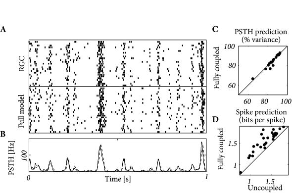
How accurate are the predictions of the multi-neuron model? Figure 11.8 describes the prediction performance. The spike trains and PSTHs of the real and modeled neurons are similar. The spike train likelihood reaches 2 bits per spike and the PSTH is predicted with 80-93% accuracy. Overall, the coupled model appears as a valid description of neurons embedded in a network.

Pillow et al. (399) also asked about the relevance of coupling between neurons. Are the coupling functions an essential part of the model or can the activity be accurately predicted without them? Optimizing the model with and without the coupling function independently, they found that the prediction of PSTH variance was unaffected. The spike prediction performance, however, showed a consistent improvement for the coupled model. (See (536) for further analysis using a model incorporating unobserved common noise effects.) Inter-neuron coupling played a greater role in decoding as we will see in the next section.