12 Neuronal Populations 12.3 Connectivity Schemes 12.5 Summary

12.4 From Microscopic to Macroscopic

In this section we will give a first example of how to make the transition from the properties of single spiking neurons to the population activity in a homogeneous group of neurons. We focus here on stationary activity.

In order to understand the dynamic response of a population of neurons to a changing stimulus, as well as for an analysis of the stability of the dynamics with respect to oscillations or perturbations, we will need further mathematical tools to be developed in the next two chapters. As we will see in Chapters 13 and 14, the dynamics depends, apart from the coupling, also on the specific choice of neuron model. However, if we want to predict the level of stationary activity in a large network of neurons, that is, if we do not worry about the temporal aspects of population activity, then the knowledge of the single-neuron gain function (f-I curve, or frequency-current relation) is completely sufficient to predict the population activity.

Fig. 12.13: The essence of a mean-field argument. A. A fully connected population of neurons (not all connections are shown). An arbitrary neuron in the network is marked as $i$ . B. Neuron $i$ has been pulled out of the network so as to show that it receives input spikes from the whole population. Hence it is driven by the population activity $A(t)$ . The same is true for all other neurons.

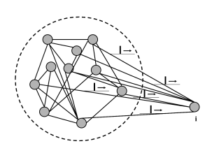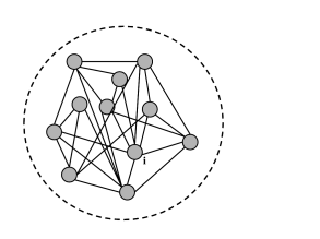
The basic argument is the following (Fig. 12.13). In a homogeneous population, each neuron receives input from many others, either from the same population, or from other populations, or both. Thus, a single neuron takes as its input a large (and in the case of a fully connected network even a complete) sample of the momentary population activity $A(t)$ . This has been made explicit in Eq. (12.4) for a single population and in Eq. (12.11) for multiple populations. To keep the arguments simple, we focus in the following on a single fully connected population. In a homogeneous population, no neuron is different from any other one, so that all neurons in the network receive the same input.

Moreover, under the assumption of stationary network activity, the neurons can be characterized by a constant mean firing rate. In this case, the population activity $A(t)$ must be directly related to the constant single-neuron firing rate $\nu$ . We show in Section 12.4.2, that, in a homogeneous population, the two are in fact equal: $A(t)=\nu$ . We emphasize that the argument sketched here and in the next paragraphs is completely independent of the choice of neuron model and holds for detailed biophysical models of the Hodgkin-Huxley type just as well as for an adaptive exponential integrate-and-fire model or a spike response model with escape noise. The argument for the stationary activity will now be made more precise.

12.4.1 Stationary activity and asynchronous firing

We define asynchronous firing of a neuronal population as a macroscopic firing state with constant activity $A(t)=A_{0}$ . In this section we show that in a homogeneous population such asynchronous firing states exist and derive the value $A_{0}$ from the properties of a single neuron. In fact, we will see that the the only relevant single-neuron property is its gain function, i.e. its mean firing rate as a function of input. More specifically, we will show that the knowledge of the gain function $g(I_{0})$ of a single neuron and the coupling parameter $J_{0}$ is sufficient to determine the activity $A_{0}$ during asynchronous firing.

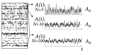
Fig. 12.14: Asynchronous firing. The empirical population activity $A(t)$ , defined as an average over the spikes across a group of $N$ neurons can be plotted after smoothing spikes with a filter $\gamma(s)$ (here the filter is exponential). In the state of stationary asynchronous activity, the filtered population activity converges toward a constant value $A_{0}$ , if the size $N$ of the group is increased (top: $N=5$ ; middle $N=10$ ; bottom $N=100$ ).

At a first glance it might look absurd to search for a constant activity $A(t)=A_{0}$ , because the population activity has been defined in Eq. (12.1) as a sum over $\delta$ -functions. Empirically the population activity is determined as the spike count across the population in a finite time interval $\Delta t$ or, more generally, after smoothing the $\delta$ -functions of the spikes with some filter. If the filter is kept fixed, while the population size is increased, the population activity in the stationary state of asynchronous firing approaches the constant value $A_{0}$ (Fig. 12.14). This argument will be made more precise below.

12.4.2 Stationary Activity as Single-Neuron Firing Rate

The population activity $A_{0}$ is equal to the mean firing rate $\nu_{i}$ of a single neuron in the population. This result follows from a trivial counting argument and can best be explained by a simple example. Suppose that in a homogeneous population of $N=$ 1 000 neurons we observe over a time $T=10s$ a total number of 25’000 spikes. Under the assumption of stationary activity $A(t)=A_{0}$ the total number of spikes is $A_{0}\,N\,T$ so that the population firing rate is $A_{0}=2.5$ Hz. Since all 1 000 neurons are identical and receive the same input, the total number of 25’ 000 spikes corresponds to 25 spikes per neuron, so that the firing rate (spike count divided by measurement time) of a single neuron $i$ is $\nu_{i}=2.5$ Hz. Thus $A_{0}=\nu_{i}$ .

More generally, the assumption of stationarity implies that averaging over time yields, for each single neuron, a good estimate of the firing rate $\nu_{0}$ . The assumption of homogeneity implies that all neurons in the population have the same parameters and are statistically indistinguishable. Therefore a spatial average across the population and the temporal average give the same result:

A_{0}=\nu_{i}\,,

(12.17)

where the index $i$ refers to the firing rate of a single, but arbitrary neuron.

For an infinitely large population, Eq. (12.17) gives a formula to predict the population activity in the stationary state. However, real populations have a finite size $N$ and each neuron in the population fires at moments determined by its intrinsic dynamics and possibly some intrinsic noise. The population activity $A(t)$ has been defined in Eq. (12.1) as an empirically observable quantity. In a finite population, the empirical activity fluctuates and we can, with the above arguments, only predict its expectation value

\langle A_{0}\rangle=\nu_{i}\,.

(12.18)

The neuron models discussed in Parts I and II enable us to calculate the mean firing rate $\nu_{i}$ for a stationary input, characterized by a mean $I_{0}$ and, potentially, fluctuations or noise of amplitude $\sigma$ . The mean firing rate is given by the gain function

\nu_{i}=g_{\sigma}(I_{0})\,,

(12.19)

where the subscript $\sigma$ is intended to remind the reader that the shape of the gain function depends on the level of noise (see Section 12.2.2). Thus, considering the pair of equations (12.18) and (12.19), we may conclude that the expected population activity in the stationary state can be predicted from the properties of single neurons.

Example: Theory vs. Simulation, Expectation vs. Observation

How can we compare the population activity $\langle A_{0}\rangle$ calculated in Eq. (12.18) with simulation results? How can we check whether a population is in a stationary state of asynchronous firing? In a simulation of a population containing a finite number $N$ of spiking neurons, the observed activity fluctuates. Formally, the (observable) activity $A(t)$ has been defined in Eq. (12.1) as a sum over $\delta$ functions. The activity $\langle A_{0}\rangle$ predicted by the theory is the expectation value of the observed activity. Mathematically speaking, the observed activity $A$ converges for $N\to\infty$ in the weak topology to its expectation value. More practically this implies that we should convolve the observed activity with a continuous test function $\gamma(s)$ before comparing with $A_{0}$ . We take a function $\gamma$ with the normalization $\int_{0}^{s^{\rm max}}\gamma(s)\,{\text{d}}s=1$ . For the sake of simplicity we assume furthermore that $\gamma$ has finite support so that $\gamma(s)=0$ for $s<0$ or $s>s^{\rm max}$ . We define

\overline{A}(t)=\int_{0}^{s^{\rm max}}\gamma(s)\,A(t-s)\,{\text{d}}s\,.

(12.20)

The firing is asynchronous if the averaged fluctuations $\langle|\overline{A}(t)-A_{0}|^{2}\rangle$ decrease with increasing $N$ ; cf. Fig. 12.14.

In order to keep the notation light, we normally write in this book simply $A(t)$ even in places where it would be more precise to write $\langle A(t)\rangle$ (the expected population activity at time $t$ , calculated by theory) or $\overline{A}(t)$ (the filtered population activity, derived from empirical measurement in a simulation or experiment). Only at places where the distinction between $A$ , $\overline{A}$ , and $\langle A\rangle$ is crucial, we use the explicit notation with bars or angle-signs.

12.4.3 Activity of a fully connected network

The gain function of a neuron is the firing rate $\nu$ as a function of its input current $I$ . In the previous subsection, we have seen that the firing rate is equivalent to the expected value of the population activity $A_{0}$ in the state of asynchronous firing. We thus have

\langle A_{0}\rangle=g_{\sigma}(I)\,.

(12.21)

The gain function in the absence of any noise (fluctuation amplitude $\sigma=0$ ) will be denoted by $g_{0}$ .

Recall that the total input $I$ to a neuron of a fully connected population consists of the external input $I^{\rm ext}(t)$ and a component that is due to the interaction of the neurons within the population. We copy Eq. (12.4) to have the explicit expression of the input current

I(t)=w_{0}\,N\int_{0}^{\infty}\alpha(s)\,A(t-s)\,{\text{d}}s+I^{\rm ext}(t)\,.

(12.22)

Since the overall strength of the interaction is set by $w_{0}$ , we can impose a normalization $\int_{0}^{\infty}\alpha(s)\,{\text{d}}s=1$ . We now exploit the assumption of stationarity and set $\int_{0}^{\infty}\alpha(s)\,A(t-s)\,{\text{d}}s=A_{0}$ . The left-hand side is the filtered observed quantity which is in reality never exactly constant, but if the number $N$ of neurons in the network is sufficiently large, we do not have to worry about small fluctuations around $A_{0}$ . Note that $\alpha$ here plays the role of the test function introduced in the previous example.

Therefore, the assumption of stationary activity $A_{0}$ combined with the assumption of constant external input $I^{\rm ext}(t)=I^{\rm ext}_{0}$ yields a constant total driving current

I_{0}=w_{0}\,N\,A_{0}+I^{\rm ext}_{0}\,.

(12.23)

Together with Eq. (12.21) we arrive at an implicit equation for the population activity $A_{0}$ ,

A_{0}=g_{0}\left({J_{0}}\,A_{0}+I_{0}^{\rm ext}\right)\,.

(12.24)

where $g_{0}$ is the noise-free gain function of single neurons and $J_{0}=w_{0}\,N$ . In words, the population activity in a homogeneous network of neurons with all-to-all connectivity can be calculated if we know the single-neuron gain function $g_{0}$ and the coupling strength $J_{0}$ . This is the central result of this section, which is independent of any specific assumption about the neuron model.

A graphical solution of Eq. (12.24) is indicated in Figure 12.15 where two functions are plotted: First, the mean firing rate $\nu=g_{0}(I_{0})$ as a function of the input $I_{0}$ (i.e., the gain function). Second, the population activity $A_{0}$ as a function of the total input $I_{0}$ (i.e., $A_{0}=[I_{0}-I^{\rm ext}_{0}]/J_{0}$ ; see Eq. (12.23)). The intersections of the two functions yield fixed points of the activity $A_{0}$ .

Fig. 12.15: Graphical solution for the fixed point $A_{0}$ of the activity in a population of spiking neurons. The intersection of the gain function $A_{0}=g_{0}(I_{0})$ (solid line) with the straight line $A_{0}=[I_{0}-I^{\rm ext}_{0}]/J_{0}$ (dotted) gives the value of the activity $A_{0}$ . Depending on the parameters, several solutions may coexist (long-dashed line).

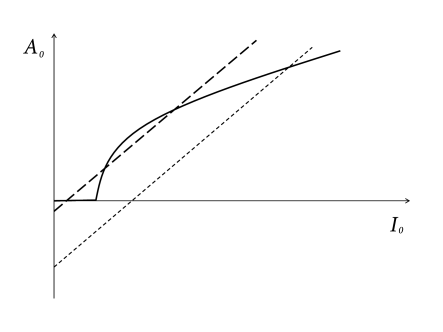
As an aside we note that the graphical construction is identical to that of the Curie-Weiss theory of ferromagnetism which can be found in any physics textbook. More generally, the structure of the equations corresponds to the mean-field solution of a system with feedback. As shown in Fig. 12.15, several solutions may coexist. We cannot conclude from the figure, whether one or several solutions are stable. In fact, it is possible that all solutions are unstable. In the latter case, the network leaves the state of asynchronous firing and evolves toward an oscillatory state. The stability analysis of the asynchronous state requires equations for the population dynamics, which will be discussed in Chapters 13 and 14.

The parameter $J_{0}$ introduced above in Eq. (12.24) implies, at least implicitly, a scaling of weights $w_{ij}=J_{0}/N$ - as suggested earlier during the discussion of fully connected networks; cf. Eq. (12.6). The scaling with $1/N$ enables us to consider the limit of a large number of neurons: if we keep $J_{0}$ fixed the equation remains the same, even if $N$ increases. Because fluctuations of the observed population activity $A(t)$ around $A_{0}$ decrease as $N$ increases, Eq. (12.24) becomes exact in the limit of $N\to\infty$ .

Example: Leaky integrate-and-fire model with diffusive noise

We consider a large and fully connected network of identical leaky integrate-and-fire neurons with homogeneous coupling $w_{ij}=J_{0}/N$ and normalized postsynaptic currents ( $\int_{0}^{\infty}\alpha(s)ds=1$ ). In the state of asynchronous firing, the total input current driving a typical neuron of the network is then

I_{0}=I^{\rm ext}_{0}+J_{0}\,A_{0}\,.\,

(12.25)

In addition, each neuron receives individual diffusive noise of variance $\sigma^{2}$ that could represent spike arrival from other populations. The single-neuron gain function (476) in the presence of diffusive noise has already been stated in Chapter 8; cf. Eq. (8.54). We use the formula of the gain function to calculate the population activity

A_{0}=g_{\sigma}(I_{0})=\left\{\tau_{m}\sqrt{\pi}\int_{{u_{r}-RI_{0}\over% \sigma}}^{{\vartheta-RI_{0}\over\sigma}}{\text{d}}u\,\exp\left(u^{2}\right)\,% \left[1+{\rm erf}(u)\right]\right\}^{-1}\,,

(12.26)

where $\sigma$ with units of voltage measures the amplitude of the noise. The fixed points for the population activity are once more determined by the intersections of these two functions; cf. Fig. 12.16.

Fig. 12.16: Graphical solution for the fixed point $A_{0}$ in the case of a fully connected network of leaky integrate-and-fire neurons. The solid lines show the single-neuron firing rate as a function of the constant input current $I_{0}$ for four different noise levels, viz. $\sigma=1.0,\sigma=0.5,\sigma=0.1,\sigma=0.0$ (from top to bottom). The intersection of the gain function with the dashed line with slope $1/J_{0}$ gives solutions for the stationary activity $A_{0}$ in a population with excitatory coupling $J_{0}$ . Other parameters: $\vartheta=1$ , $R=1$ , $\tau=10$ ms.

12.4.4 Activity of a randomly connected network

In the preceding subsections we have studied the stationary state of a large population of neurons for a given noise level. In Fig. 12.16 the noise was modeled explicitly as diffusive noise and can be interpreted as the effect of stochastic spike arrival from other populations or some intrinsic noise source inside each neuron. In other words, noise was added explicitly to the model while the input current $I_{i}(t)$ to neuron $i$ arising from other neurons in the population was constant and the same for all neurons: $I_{i}=I_{0}$ .

In a randomly connected network (and similarly in a fully connected network of finite size), the summed synaptic input current arising from other neurons in the population is, however, not constant but fluctuates around a mean value $I_{0}$ , even if the population is in a stationary state of asynchronous activity. In this subsection, we discuss how to mathematically treat the additional noise arising from the network.

We assume that the network is in a stationary state where each neuron fires stochastically, independently, and at a constant rate $\nu$ , so that the firing of different neurons exhibits only chance coincidences. Suppose that we have a randomly connected network of $N$ neurons where each neuron receives input from $C_{\rm pre}$ presynaptic partners. All weights are set equal to $w_{ij}=w$ .

We are going to determine the firing rate $\nu=A_{0}$ of a typical neuron in the network self-consistently as follows. If all neurons fire at a rate $\nu$ then the mean input current to neuron $i$ generated by its $C_{\rm pre}$ presynaptic partners is

\langle I_{0}\rangle=C_{\rm pre}\,q\,w\,\nu+I^{\rm ext}_{0}\,,

(12.27)

where $q=\int_{0}^{\infty}\alpha(s)\,{\text{d}}s$ denotes the integral over the postsynaptic current and can be interpreted as the total electric charge delivered by a single input spike; cf. Section 8.2 in Chapter 8.

The input current is not constant but fluctuates with a variance $\sigma_{I}^{2}$ given by

\sigma_{I}^{2}=C_{\rm pre}\,w^{2}\,q_{2}\,\nu\,,

(12.28)

where $q_{2}=\int_{0}^{\infty}\alpha^{2}(s)\,{\text{d}}s$ ; see Section 8.2 in Chapter 8.

Thus, if neurons fire at constant rate $\nu$ , we know the mean input current and its variance. In order to close the argument we use the single-neuron gain function

\nu=g_{\sigma}(I_{0})\,.

(12.29)

which is supposed to be known for arbitrary noise levels $\sigma_{I}$ . If we insert the mean $I_{0}$ from Eq. (12.27) and its standard deviation $\sigma_{I}$ from Eq. (12.28), we arrive at an implicit equation for the firing rate $\nu$ which we need to solve numerically. The mean population activity is then $\langle A_{0}\rangle=\nu$ .

We emphasize that the above argument does not require any specific neuron model. In fact, it holds for biophysical neuron models of the Hodgkin-Huxley type as well as for integrate-and-fire models. The advantage of a leaky integrate-and-fire model is that an explicit mathematical formula for the gain function $g_{\sigma}(I_{0})$ is available. An example will be given below. But we can use Eqs. (12.27) - (12.29) just as well for a homogeneous population of biophysical neuron models. The only difference is that we have to numerically determine the single-neuron gain function $g_{\sigma}(I_{0})$ for different noise levels (with noise of the appropriate autocorrelation) before starting to solve the network equations.

Please also note that the above argument is not restricted to a network consisting of a single population. It can be extended to several interacting populations. In this case, the expressions for the mean and variance of the input current contain contributions from the other populations, as well as from the self-interaction in the network. An example with interacting excitatory and inhibitory populations is given below.

The arguments that have been developed above for networks with a fixed number of presynaptic partners $C_{\rm pre}$ can also be generalized to networks with asymmetric random connectivity of fixed connection probability $p$ and synaptic scaling $w_{ij}=J_{0}/\sqrt{N}$ (15; 487; 91; 532; 487; 44).

Brunel network: excitatory and inhibitory populations

The self-consistency argument will now be applied to the case of two interacting populations, an excitatory population with $N_{E}$ neurons and an inhibitory population with $N_{I}$ neurons. The neurons in both populations are modeled by leaky integrate-and-fire neurons. For the sake of convenience, we set the resting potential to zero ( $u_{\rm rest}=0$ ). We have seen in Chapter 8 that leaky integrate-and-fire neurons with diffusive noise generate spike trains with a broad distribution of interspike intervals when they are driven in the sub-threshold regime. We will use this observation to construct a self-consistent solution for the stationary states of asynchronous firing.

We assume that excitatory and inhibitory neurons have the same parameters $\vartheta$ , $\tau_{m}$ , $R$ , and $u_{r}$ . In addition, all neurons are driven by a common external current $I^{\rm ext}$ . Each neuron in the population receives $C_{E}$ synapses from excitatory neurons with weight $w_{E}>0$ and $C_{I}$ synapses from inhibitory neurons with weight $w_{I}<0$ . If an input spike arrives at the synapses of neuron $i$ from a presynaptic neuron $j$ , its membrane potential changes by an amount $\Delta u_{E}=w_{E}\,q\,R/\tau_{m}$ if $j$ is excitatory and $\Delta u_{I}=\Delta u_{E}\,w_{I}/w_{E}$ if $j$ is inhibitory. Here $q$ has units of electric charge. We set

\gamma={C_{I}\over C_{E}}\quad\text{ and }\quad g=-{w_{I}\over w_{E}}=-{\Delta u% _{I}\over\Delta u_{E}}\,.

(12.30)

Since excitatory and inhibitory neurons receive the same number of input connections in our model, we assume that they fire with a common firing rate $\nu$ . The total input current generated by the external current and by the lateral couplings is

	$\displaystyle I_{0}$	$\displaystyle=$	$\displaystyle I^{\rm ext}+q\,\sum_{j}\nu_{j}\,w_{j}$		(12.31)
		$\displaystyle=$	$\displaystyle I_{0}^{\rm ext}+q\,\nu\,w_{E}\,C_{E}\,[1-\gamma\,g]\,.$		(12.31)

Because each input spike causes a jump of the membrane potential, it is convenient to measure the noise strength by the variance $\sigma^{2}_{u}$ of the membrane potential (as opposed to the variance $\sigma^{2}_{I}$ of the input). With the definitions of Chapter 8, we set $\sigma_{u}^{2}=0.5\sigma^{2}$ where, from Eq. (8.42),

	$\displaystyle\sigma^{2}$	$\displaystyle=$	$\displaystyle\sum_{j}\nu_{j}\,\tau\,(\Delta u_{j}^{2})$		(12.32)
		$\displaystyle=$	$\displaystyle\nu\,(\Delta u_{E})^{2}\,C_{E}\,[1+\gamma\,g^{2}]\,.$		(12.32)

The stationary firing rate $A_{0}$ of the population with mean input $I_{0}$ and variance $\sigma$ is copied from Eq. (12.26) and repeated here for convenience

A_{0}=\nu=g_{\sigma}(I_{0})={1\over\tau_{m}}\left\{{\sqrt{\pi}}\int_{{u_{r}-RI% _{0}\over\sigma}}^{{\vartheta-RI_{0}\over\sigma}}\,\exp\left({x}^{2}\right)\,% \left[1+{\rm erf}(x)\right]\,{\text{d}}x\right\}^{-1}\,.

(12.33)

In a stationary state we must have $A_{0}=\nu$ . To get the value of $A_{0}$ we must therefore solve Eqs. (12.31) – (12.33) simultaneously for $\nu$ and $\sigma$ . Since the gain function, i.e., the firing rate as a function of the input $I_{0}$ depends on the noise level $\sigma$ , a simple graphical solution as in Fig. 12.15 is no longer possible. Numerical solutions of Eqs. (12.31) – (12.33) have been obtained by Amit and Brunel (21, 20). For a mixed graphical-numerical approach see Mascaro and Amit (332).

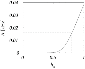
In the following paragraphs we give some examples of how to construct self-consistent solutions. For convenience we always set $\vartheta=1$ , $q=1$ , $R=1$ and $\tau_{m}=10$ ms and work with a unit-free current $I\to h$ . Our aim is to find connectivity parameters such that the mean input to each neuron is $h=0.8$ and its variance $\sigma=0.2$ .

Figure 12.17A shows that $h_{0}=0.8$ and $\sigma=0.2$ correspond to a firing rate of $A_{0}=\nu\approx 16\,$ Hz. We set $\Delta u_{E}=0.025$ , i.e., 40 simultaneous spikes are necessary to make a neuron fire. Inhibition has the same strength $w_{I}=-w_{E}$ so that $g=1$ . We constrain our search to solutions with $C_{E}=C_{I}$ so that $\gamma=1$ . Thus, on the average, excitation and inhibition balance each other. To get an average input potential of $h_{0}=0.8$ we therefore need a constant driving current $I^{\rm ext}=0.8$ .

To arrive at $\sigma=0.2$ we solve Eq. (12.32) for $C_{E}$ and find $C_{E}=C_{I}=200$ . Thus for this choice of the parameters the network generates enough noise to allow a stationary solution of asynchronous firing at 16 Hz.

Fig. 12.17: A. Mean activity of a population of integrate-and-fire neurons with diffusive noise amplitude of $\sigma=0.2$ as a function of $h_{0}=R\,I_{0}$ . For $h_{0}=0.8$ the population rate is $\nu\approx 16$ Hz (dotted line). B. Mean activity of a population of integrate-and-fire neurons with diffusive noise of $\sigma=0.54$ as a function of $h_{0}=R\,I_{0}$ . For $h_{0}=0.2$ the population rate is $\nu=8$ Hz (dotted line). The long-dashed line shows $A_{0}=[h_{0}-h_{0}^{\rm ext}]/J^{\rm eff}$ with an effective coupling $J^{\rm eff}<0$ .

Note that, for the same parameters, the inactive state where all neurons are silent is also a solution. Using the methods discussed in this section we cannot say anything about the stability of these states. For the stability analysis see Chapter 13.

Example: Inhibition dominated network

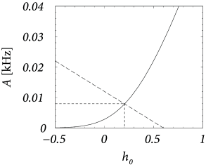
About eighty to ninety percent of the neurons in the cerebral cortex are excitatory and the remaining ten to twenty percent inhibitory. Let us suppose that we have $N_{E}=$ 8 000 excitatory and $N_{I}=$ 2 000 inhibitory neurons in a cortical column. We assume random connectivity with a connection probability of ten percent and take $C_{E}=800$ , $C_{I}=200$ so that $\gamma=1/4$ . As before, spikes arriving at excitatory synapses cause a voltage jump $\Delta u_{E}=0.025$ , i.e, an action potential can be triggered by the simultaneous arrival of 40 presynaptic spikes at excitatory synapses. If neurons are driven in the regime close to threshold, inhibition is rather strong and we take $\Delta u_{I}=-0.125$ so that $g=5$ . Even though we have less inhibitory than excitatory neurons, the mean feedback is then dominated by inhibition since $\gamma\,g>1$ . We search for a consistent solution of Eqs. (12.31) – (12.33) with a spontaneous activity of $\nu=8$ Hz.

Given the above parameters, the variance is $\sigma\approx 0.54$ ; cf. Eq. (12.32). The gain function of integrate-and-fire neurons gives us for $\nu=8$ Hz a corresponding total potential of $h_{0}\approx 0.2$ ; cf. Fig. 12.17B. To attain $h_{0}$ we have to apply an external stimulus $h_{0}^{\rm ext}=R\,I^{\rm ext}$ which is slightly larger than $h_{0}$ since the net effect of the lateral coupling is inhibitory. Let us introduce the effective coupling $J^{\rm eff}=\tau\,C_{E}\,\Delta u_{E}\,(1-\gamma\,g)$ . Using the above parameters we find from Eq. (12.31) $h_{0}^{\rm ext}=h_{0}-J^{\rm eff}\,A_{0}\approx 0.6$ .

The external input could, of course, be provided by (stochastic) spike arrival from other columns in the same or other areas of the brain. In this case Eq. (12.31) is to be replaced by

h_{0}=\tau_{m}\,\nu\,\Delta u_{E}\,C_{E}\,[1-\gamma\,g]\,+\tau_{m}\,\nu_{\rm ext% }\Delta u_{\rm ext}\,C_{\rm ext}\,,

(12.34)

with $C_{\rm ext}$ the number of connections that a neuron receives from neurons outside the population, $\Delta u_{\rm ext}$ their typical coupling strength characterized by the amplitude of the voltage jump, and $\nu_{\rm ext}$ their spike arrival rate (21; 20). Due to the extra stochasticity in the input, the variance $\sigma_{u}^{2}$ of the membrane voltage is larger

\sigma_{u}^{2}=0.5\sigma^{2}=0.5\tau_{m}\,\nu\,(\Delta u_{E})^{2}\,C_{E}\,[1+% \gamma\,g^{2}]+0.5\tau_{m}\,\nu_{\rm ext}(\Delta u_{\rm ext})^{2}\,C_{\rm ext}

(12.35)

The equations (12.33), (12.34) and (12.35) can be solved numerically (21; 20). The analysis of the stability of the solution is slightly more involved (78; 79), and will be considered in Chapter 13.

Example: Vogels-Abbott network

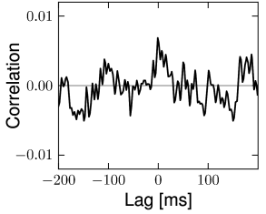
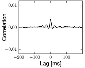
The structure of the network studied by Vogels and Abbott (537; 538; 68) is the same as that for the Brunel network: excitatory and inhibitory model neurons have the same parameters and are connected with the same probability $p$ within and across the two sup-populations. Therefore inhibitory and excitatory neurons fire with the same mean firing rate (see Section 12.4.4) and with hardly any correlations above chance level (Fig. 12.18). The two main differences to the Brunel network are: (i) the choice of random connectivity in the Vogels-Abbott network does not preserve the number of presynaptic partners per neuron so that some neurons receive more and others less than $pN$ connections; (ii) neurons in the Vogels-Abbott network communicate with each other by conductance-based synapses. A spike fired at time $t_{j}^{(f)}$ causes a change in conductance

\tau_{g}{dg\over dt}=-g+\tau_{g}\Delta g\sum_{f}\delta(t-t_{j}^{(f)})\,.

(12.36)

Thus, a synaptic input causes for $t>t_{j}^{(f)}$ a contribution to the conductance $g(t)=\Delta g\,\exp[-(t-t_{j}^{(f)})/\tau_{g}]$ . The neurons are leaky integrate-and-fire units.

As will be discussed in more detail in Section 13.6.3 of the next chapter, the dominant effect of conductance based input is a decrease of the effective membrane time constant. In other words, if we consider a network of leaky integrate-and-fire neurons (with resting potential $u_{\rm rest}=0$ ), we may use again the Siegert-formula of Eq. (12.26)

A_{0}=g_{\sigma}(I_{0})=\left\{\tau_{\rm eff}(I_{0},\sigma)\sqrt{\pi}\int_{{u_% {r}-RI_{0}\over\sigma}}^{{\vartheta-RI_{0}\over\sigma}}{\text{d}}u\,\exp\left(% u^{2}\right)\,\left[1+{\rm erf}(u)\right]\right\}^{-1}\,,

(12.37)

in order to calculate the population activity $A_{0}$ . The main difference to the current-based model is that the mean input current $I_{0}$ and the fluctuations $\sigma$ of the membrane voltage now also enter into the time constant $\tau_{\rm eff}$ . The effective membrane time constant $\tau_{\rm eff}$ in simulations of conductance-based integrate-and-fire neurons is sometimes four or five times shorter than the raw membrane time constant $\tau_{m}$ (126; 537; 538).

The Siegert formula holds in the limit of short synaptic time constants ( $\tau_{E}\to 0$ and $\tau_{I}\to 0$ ). The assumption of short time constants for the conductances is necessary, because the Siegert formula is valid for white noise, corresponding to short pulses. However, the gain function of integrate-and-fire neurons for colored diffusive noise can also be determined (154); see Section 13.6.4 of Chapter 13.

Fig. 12.18: Pairwise correlation of neurons in the Vogels-Abbott network. A. Excess probability of observing a spike in a neuron $i$ at time $t$ and a spike in neuron $j$ at time $t^{\prime}$ for various time lags $t-t^{\prime}$ , after subtraction of chance coincidences. Normalization such that two identical spike trains would give a value of one at zero time lag. B As in A, but averaged across 171 randomly chosen pairs. The pairwise correlations are extremely small in this randomly connected network of 8000 excitatory and 2000 inhibitory neurons with connection probability $p=0.02$ and conductance-based synapses; see (539) for details. Mean firing rate is $A_{0}=5$ Hz.

12.4.5 Apparent stochasticity and chaos in a deterministic network

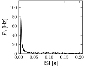
In this section we discuss how a network of deterministic neurons with fixed random connectivity can generate its own noise. In particular, we will focus on spontaneous activity and argue that there exist stationary states of asynchronous firing at low firing rates which have broad distributions of interspike intervals (Fig. 12.19) even though individual neurons are deterministic. The arguments made here have tacitly been used throughout Section 12.4.

Fig. 12.19: Interspike interval distributions in the Vogels-Abbott network. A. Interspike interval distribution of a randomly chosen neuron. Note the long tail of the distribution. The width of the distribution can be characterized by a coefficient of variation of $CV=1.9$ . B. Distribution of the CV index across all 10 000 neurons of the network. Bin width of horizontal axis is 0.01.

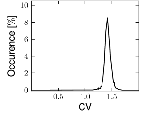Van Vreeswijk and Sompolinsky (1996, 1998) used a network of binary neurons to demonstrate broad interval distribution in deterministic networks. Amit and Brunel (21, 20) were the first to analyze a network of integrate-and-fire neurons with fixed random connectivity. While they allowed for an additional fluctuating input current, the major part of the fluctuations were in fact generated by the network itself. The theory of randomly connected integrate-and-fire neurons has been further developed by Brunel and Hakim (78). In a later study, Brunel (79) confirmed that asynchronous highly irregular firing can be a stable solution of the network dynamics in a completely deterministic network consisting of excitatory and inhibitory integrate-and-fire neurons. Work of Tim Vogels and Larry Abbott has shown that asynchronous activity at low firing rates can indeed be observed reliably in networks of leaky integrate-and-fire neurons with random coupling via conductance-based synapses (537; 538; 68). The analysis of randomly connected networks of integrate-and-fire neurons (79) is closely related to earlier theories for random nets of formal analog or binary neurons (15; 16; 17; 278; 368; 107; 91). However, the reset of neurons after each spike can be the cause of additional instabilities that have been absent in these earlier networks with analog or binary neurons.

Random connectivity of the network plays a central role in the arguments. We focus on randomness with a fixed number $C$ of presynaptic partners. Sparse connectivity means that the ratio

\delta={C\over N}\ll 1

(12.38)

is a small number. Formally, we may take the limit of $N\to\infty$ while keeping $C$ fixed. As a consequence of the sparse random network connectivity two neurons $i$ and $j$ share only a small number of common inputs. In the limit of $C/N\to 0$ the probability that neurons $i$ and $j$ have a common presynaptic neuron vanishes. Thus, if the presynaptic neurons fire stochastically, then the input spike trains that arrive at neuron $i$ and $j$ are independent (123; 278). In that case, the input of neuron $i$ and $j$ can be described as uncorrelated stochastic spike arrival which in turn can be approximated by a diffusive noise model; cf. Chapter 8. Therefore, in a large and suitably constructed random network, correlations between spiking neurons can be arbitrarily low (426); cf. Fig. 12.18.

Note that this is in stark contrast to a fully connected network of finite size where neurons receive highly correlated input, but the correlations are completely described by the time course of the population activity.