8 Noisy Input Models: Barrage of Spike Arrivals 8.3 Subthreshold vs. Superthreshold regime 8.5 Summary

8.4 Diffusion limit and Fokker-Planck equation(*)

In this section we analyze the model of stochastic spike arrival defined in Eq. (8.20) and show how to map it to the diffusion model defined in Eq. (8.7) (190; 243; 88). Suppose that the neuron has fired its last spike at time $\hat{t}$ . Immediately after the firing the membrane potential was reset to $u_{r}$ . Because of the stochastic spike arrival, we cannot predict the membrane potential for $t>\hat{t}$ , but we can calculate its probability density, $p(u,t)$ . The evolution of the probability density as a function of time is described, in the diffusion limit, by the Fokker-Planck equation which we derive here in the context of a single neuron subject to noisy input. In part III (Chapter 13.1.1) the Fokker-Planck equation will be introduced systematically in the context of populations of neurons.

For the sake of simplicity, we set for the time being $I^{\rm ext}=0$ in Eq. (8.20). The input spikes at synapse $k$ are generated by a Poisson process and arrive stochastically with rate $\nu_{k}(t)$ . The probability that no spike arrives in a short time interval $\Delta t$ is therefore

{\rm Prob}\big\{{\rm no~{}spike~{}in~{}}[t,t+\Delta t]\big\}=1-\sum_{k}\nu_{k}% (t)\,\Delta t\,.

(8.36)

If no spike arrives in $[t,t+\Delta t]$ , the membrane potential changes from $u(t)=u^{\prime}$ to $u(t+\Delta t)=u^{\prime}\,\exp(-\Delta t/\tau_{m})$ . On the other hand, if a spike arrives at synapse $k$ , the membrane potential changes from $u^{\prime}$ to $u^{\prime}\,\exp(-\Delta t/\tau_{m})+w_{k}$ . Given a value of $u^{\prime}$ at time $t$ , the probability density of finding a membrane potential $u$ at time $t+\Delta t$ is therefore given by

	$\displaystyle P^{\rm trans}(u,t+\Delta t\|u^{\prime},t)$	$\displaystyle=$	$\displaystyle\big[1-\Delta t\sum_{k}\nu_{k}(t)\big]\,\delta\left(u-u^{\prime}% \,e^{-\Delta t/\tau_{m}}\right)$		(8.37)
			$\displaystyle+\Delta t\sum_{k}\nu_{k}(t)\delta\left(u-u^{\prime}\,e^{-\Delta t% /\tau_{m}}-w_{k}\right)\,.$		(8.37)

We will refer to $P^{\rm trans}$ as the transition law. Since the membrane potential is given by the differential equation (8.20) with input spikes generated by a Poisson distribution, the evolution of the membrane potential is a Markov Process (i.e., a process without memory) and can be described by (529)

p(u,t+\Delta t)=\int P^{\rm trans}(u,t+\Delta t|u^{\prime},t)\,p(u^{\prime},t)% \,{\text{d}}u^{\prime}\,.

(8.38)

We insert Eq. (8.37) in Eq. (8.38). To perform the integration, we have to recall the rules for $\delta$ functions, viz., $\delta(a\,u)=a^{-1}\,\delta(u)$ . The result of the integration is

	$\displaystyle p(u,t+\Delta t)$	$\displaystyle=$	$\displaystyle\big[1-\Delta t\sum_{k}\nu_{k}(t)\big]\,e^{\Delta t/\tau_{m}}\,p% \left(e^{\Delta t/\tau_{m}}\,u,t\right)$		(8.39)
			$\displaystyle+\Delta t\sum_{k}\nu_{k}(t)\,e^{\Delta t/\tau_{m}}\,p\left(e^{% \Delta t/\tau_{m}}\,u-w_{k},t\right)\,.$		(8.39)

Since $\Delta t$ is assumed to be small, we expand Eq. (8.39) about $\Delta t=0$ and find to first order in $\Delta t$

	$\displaystyle{p(u,t+\Delta t)-p(u,t)\over\Delta t}$	$\displaystyle=$	$\displaystyle{1\over\tau_{m}}\,p(u,t)+{1\over\tau_{m}}\,u\,{\partial\over% \partial u}p(u,t)$		(8.40)
			$\displaystyle+\sum_{k}\nu_{k}(t)\,\left[p(u-w_{k},t)-p(u,t)\right]\,.$		(8.40)

For $\Delta t\to 0$ , the left-hand side of Eq. (8.40) turns into a partial derivative $\partial p(u,t)/\partial t$ . Furthermore, if the jump amplitudes $w_{k}$ are small, we can expand the right-hand side of Eq. (8.40) with respect to $u$ about $p(u,t)$ :

	$\displaystyle\tau_{m}{\partial\over\partial t}p(u,t)$	$\displaystyle=$	$\displaystyle-{\partial\over\partial u}\left[-u+\tau_{m}\sum_{k}\nu_{k}(t)\,w_% {k}\right]\,p(u,t)$		(8.41)
			$\displaystyle+{1\over 2}\,\left[\tau_{m}\sum_{k}\nu_{k}(t)\,w_{k}^{2}\right]\,% {\partial^{2}\over\partial u^{2}}p(u,t),$		(8.41)

where we have neglected terms of order $w_{k}^{3}$ and higher. The expansion in $w_{k}$ is called the Kramers-Moyal expansion. Eq. (8.41) is an example of a Fokker-Planck equation (529), i.e., a partial differential equation that describes the temporal evolution of a probability distribution. The right-hand side of Eq. (8.41) has a clear interpretation: The first term in rectangular brackets describes the systematic drift of the membrane potential due to leakage ( $\propto-u$ ) and mean background input ( $\propto\sum_{k}\nu_{k}(t)\,w_{k}$ ). The second term in rectangular brackets corresponds to a ‘diffusion constant’ and accounts for the fluctuations of the membrane potential. The Fokker-Planck Eq. (8.41) is equivalent to the Langevin equation (8.7) with $R\,I(t)=\tau_{m}\sum_{k}\nu_{k}(t)\,w_{k}$ and time-dependent noise amplitude

{\sigma}^{2}(t)=\,\tau_{m}\,\sum_{k}\nu_{k}(t)\,w_{k}^{2}\,.

(8.42)

The specific process generated by the Langevin-equation (8.7) with constant noise amplitude $\sigma$ is called the Ornstein-Uhlenbeck process (527), but Eq. (8.42) indicates that, in the context of neuroscience, the effective noise amplitude generated by stochastic spike arrival is in general time-dependent. We will return to the Fokker-Planck equation in Ch. 13.

For the transition from Eq. (8.40) to (8.41) we have suppressed higher-order terms in the expansion. The missing terms are

\sum_{n=3}^{\infty}{(-1)^{n}\over n!}\,A_{n}(t){\partial^{n}\over\partial u^{n% }}p(u,t)

(8.43)

with $A_{n}=\tau_{m}\sum_{k}\nu_{k}(t)\,w_{k}^{n}$ . What are the conditions that these terms vanish? As in the example of Figs. 8.6A and B, we consider a sequence of models where the size of the weights $w_{k}$ decreases so that $A_{n}\to 0$ for $n\geq 3$ while the mean $\sum_{k}\nu_{k}(t)\,w_{k}$ and the second moment $\sum_{k}\nu_{k}(t)\,w_{k}^{2}$ remain constant. It turns out, that, given both excitatory and inhibitory input, it is always possible to find an appropriate sequence of models (286; 287). For $w_{k}\to 0$ , the diffusion limit is attained and Eq. (8.41) is exact. For excitatory input alone, however, such a sequence of models does not exist (406).

8.4.1 Threshold and firing

The Fokker-Planck equation (8.41) and the Langevin equation (8.7) are equivalent descriptions of drift and diffusion of the membrane potential. Neither of these describe spike firing. To turn the Langevin equation (8.7) into a sensible neuron model, we have to incorporate a threshold condition. In the Fokker-Planck equation (8.41), the firing threshold is incorporated as a boundary condition

p(\vartheta,t)\equiv 0\,\quad{\rm for~{}all~{}}t\,.

(8.44)

The boundary condition reflects the fact that, under a white noise model, in each short interval $\Delta t$ many excitatory and inhibitory input spikes arrive which each cause a tiny jump of size $\pm\delta$ of the membrane potential. Any finite density $p(u,t)$ at a value $\vartheta-\delta<u\leq\vartheta$ would be rapidly removed, because one of the many excitatory spikes which arrive at each moment would push the membrane potential above threshold. The white noise limit corresponds to infinite spike arrival rate and jump size $\delta\to 0$ , as discussed above. As a consequence there are, in each short interval $\Delta t$ infinitely many ’attempts’ to push the membrane potential above threshold. Hence the density at $u=\vartheta$ must vanish. The above argument also shows that for colored noise the density at threshold is finite, because the the effective frequency of ’attempts’ is limited by the cut-off frequency of the noise.

Before we continue the discussion of the diffusion model in the presence of a threshold, let us study the solution of Eq. (8.41) without threshold.

Example: Free distribution

The solution of the Fokker-Planck equation (8.41) with initial condition $p(u,\hat{t})=\delta(u-u_{r})$ is a Gaussian with mean $u_{0}(t)$ and variance $\langle\Delta u^{2}(t)\rangle$ , i.e.,

p(u,t)={1\over\sqrt{2\pi\,\langle\Delta u^{2}(t)\rangle}}\,\exp\left\{-{[u(t|% \hat{t})-u_{0}(t)]^{2}\over 2\,\langle\Delta u^{2}(t)\rangle}\right\}

(8.45)

as can be verified by inserting Eq. (8.45) into (8.41). In particular, the stationary distribution that is approached in the limit of $t\to\infty$ for constant input $I_{0}$ is

p(u,\infty)={1\over\sqrt{\pi}}{1\over\sigma}\exp\left\{{[u-R\,I_{0}]^{2}\over% \sigma^{2}}\right\}\,,

(8.46)

which describes a Gaussian distribution with mean $u_{\infty}=R\,I_{0}$ and variance $\sigma/\sqrt{2}$ .

8.4.2 Interval distribution for the diffusive noise model

Let us consider a leaky integrate-and-fire neuron that starts at time $\hat{t}$ with a membrane potential $u_{r}$ and is driven for $t>\hat{t}$ by a known input $I(t)$ . Because of the diffusive noise generated by stochastic spike arrival, we cannot predict the exact value of the neuronal membrane potential $u(t)$ at a later time $t>\hat{t}$ , but only the probability that the membrane potential is in a certain interval $[u_{0},u_{1}]$ . Specifically, we have

{\rm Prob}\left\{u_{0}\!<\!u(t)\!<\!u_{1}\,|\,u(\hat{t})\!=\!u_{r}\right\}\,=% \,\int_{u_{0}}^{u_{1}}p(u,t)\,{\text{d}}u

(8.47)

where $p(u,t)$ is the probability density of the membrane potential at time $t$ . In the diffusion limit, $p(u,t)$ can be found by solution of the Fokker-Planck equation Eq. (8.41) with initial condition $p(u,\hat{t})=\delta(u-u_{r})$ and boundary condition $p(\vartheta,t)=0$ .

The boundary is absorbing. In other words, in a simulation of a single realization of the stochastic process, the simulation is stopped when the trajectory passes the threshold for the first time. To be concrete, imagine that we run 100 simulation trials, i.e., 100 realization of a leaky integrate-and-fire model with diffusive noise. Each trial starts at the same value $u(\hat{t})=u_{r}$ and uses the same input current $I(t^{\prime})$ for $t^{\prime}>\hat{t}$ . Some of the trials will exhibit trajectories that reach the threshold at some point $t^{\prime}<t$ . Others stay below threshold for the whole period $\hat{t}<t^{\prime}<t$ . The expected fraction of simulations that have not yet reached the threshold and therefore still ’survive’ up to time $t$ is given by the survivor function,

S_{I}(t|\hat{t})=\int_{-\infty}^{\vartheta}p(u,t)\,{\text{d}}u\,.

(8.48)

In other words, the survivor function in the diffusive noise model is equal to the probability that the membrane potential has not yet reached the threshold between $\hat{t}$ and $t$ .

In view of Eq. (7.24), the input-dependent interval distribution is therefore

P_{I}(t|\hat{t})=-\frac{{\text{d}}}{{\text{d}}t}\int_{-\infty}^{\vartheta}p(u,% t)\,{\text{d}}u\,.

(8.49)

We recall that $P_{I}(t|\hat{t})\,\Delta t$ for $\Delta t\to 0$ is the probability that a neuron fires its next spike between $t$ and $t+\Delta t$ given a spike at $\hat{t}$ and input $I$ . In the context of noisy integrate-and-fire neurons $P_{I}(t|\hat{t})$ is called the distribution of ‘first passage times’. The name is motivated by the fact, that firing occurs when the membrane potential crosses $\vartheta$ for the first time. Unfortunately, no general solution is known for the first passage time problem of the Ornstein-Uhlenbeck process. For constant input $I(t)=I_{0}$ , however, it is at least possible to give a moment expansion of the first passage time distribution. In particular, the mean of the first passage time can be calculated in closed form.

Fig. 8.9: Without a threshold, several trajectories can reach at time $t$ the same value $u=\vartheta$ from above or below.

Example: Numerical evaluation of $P_{I}(t|\hat{t})$

We have seen that, in the absence of a threshold, the Fokker-Planck Equation (8.41) can be solved; cf. Eq. (8.45). The transition probability from an arbitrary starting value $u^{\prime}$ at time $t^{\prime}$ to a new value $u$ at time $t$ is

P^{\rm trans}(u,t|u^{\prime},t^{\prime})={1\over\sqrt{2\pi\,\langle\Delta u^{2% }(t)\rangle}}\,\exp\left\{-{[u-u_{0}(t)]^{2}\over 2\,\langle\Delta u^{2}(t)% \rangle}\right\}

(8.50)

with

	$\displaystyle u_{0}(t)$	$\displaystyle=$	$\displaystyle u^{\prime}\,e^{-(t-t^{\prime})/\tau_{m}}+\int_{0}^{t-t^{\prime}}% e^{-s^{\prime}/\tau_{m}}\,I(t-s^{\prime})\,{\text{d}}s$		(8.51)
	$\displaystyle\langle\Delta u^{2}(t)\rangle$	$\displaystyle=$	$\displaystyle{\sigma^{2}\over 2}\left[1-e^{-2\,(t-s)/\tau_{m}}\right]\,.$		(8.52)

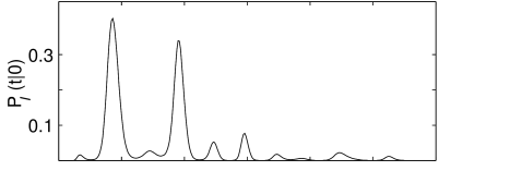
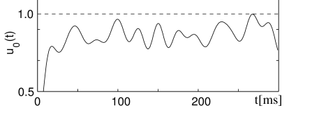
A method due to Schrödinger uses the solution of the unbounded problem in order to calculate the input-dependent interval distribution $P_{I}(t|\hat{t})$ of the diffusion model with threshold (459; 404; 83). The idea of the solution method is illustrated in Fig. 8.9. Because of the Markov property, the probability density to cross the threshold (not necessarily for the first time) at a time $t$ , is equal to the probability to cross it for the first time at $t^{\prime}<t$ and to return back to $\vartheta$ at time $t$ , that is,

P^{\rm trans}(\vartheta,t|u_{r},\hat{t})=\int_{\hat{t}}^{t}P_{I}(t^{\prime}|% \hat{t})\,P^{\rm trans}(\vartheta,t|\vartheta,t^{\prime})\,{\text{d}}t^{\prime% }\,.

(8.53)

This integral equation can be solved numerically for the distribution $P_{I}(t^{\prime}|\hat{t})$ for arbitrary input current $I(t)$ (405). An example is shown in Fig. 8.10. The probability to emit a spike is high whenever the noise-free trajectory is close to the firing threshold. Very long intervals are unlikely, if the noise-free membrane potential was already several times close to the threshold before, so that the neuron has had ample opportunity to fire earlier.

Fig. 8.10: A time-dependent input current $I(t)$ generates a noise-free membrane potential $u_{0}(t)$ shown in the lower part of the figure. In the presence of diffusive noise, spikes can be triggered although the reference trajectory stays below the threshold (dashed line). This gives rise to an input-dependent interval distribution $P_{I}(t|0)$ shown in the upper panel. Taken from (403).

8.4.3 Mean interval and mean firing rate (diffusive noise)

For constant input $I_{0}$ the mean interspike interval is $\langle s\rangle=\int_{0}^{\infty}s\,P_{I_{0}}(s|0){\text{d}}s=\int_{0}^{% \infty}s\,P_{0}(s){\text{d}}s$ ; cf. Eq. (7.13). For the diffusion model Eq. (8.7) with threshold $\vartheta$ , reset potential $u_{r}$ , and membrane time constant $\tau_{m}$ , the mean interval is

\langle s\rangle=\tau_{m}\,\sqrt{\pi}\int_{{u_{r}-h_{0}\over\sigma}}^{{% \vartheta-h_{0}\over\sigma}}{\text{d}}u\,\exp\left(u^{2}\right)\,\left[1+{\rm erf% }(u)\right]\,,

(8.54)

where $h_{0}=R\,I_{0}$ is the input potential caused by the constant current $I_{0}$ (476; 243). Here ’erf’ denotes the error function ${\rm erf}(x)=\frac{2}{\sqrt{2pi}}\int_{0}^{x}\exp(-u^{2})du$ . This expression, sometimes called the Siegert-formula, can be derived by several methods; for reviews see, e.g., (529). The inverse of the mean interval is the mean firing rate. Hence, Eq. (8.54) enables us the express the mean firing rate of a leaky integrate-and-fire model with diffusive noise as a function of a (constant) input $I_{0}$ (Fig. 8.11). We will derive Eq. (8.54) in Chapter 13 in the context of populations of spiking neurons.