19 Synaptic Plasticity and Learning 19.2 Models of Hebbian learning 19.4 Reward-based learning

19.3 Unsupervised learning

In artificial neural networks some, or even all, neurons receive input from external sources as well as from other neurons in the network. Inputs from external sources are typically described as a statistical ensemble of potential stimuli. Unsupervised learning in the field of artificial neural networks refers to changes of synaptic connections which are driven by the statistics of the input stimuli – in contrast to supervised learning or reward-based learning where the network parameters are optimized to achieve, for each stimulus, an optimal behavior. Hebbian learning rules, as introduced in the previous section, are the prime example of unsupervised learning in artificial neural networks.

In the following we always assume that there are $N$ input neurons $1\leq j\leq N$ . Their firing rates $\nu_{j}$ are chosen from a set of $P$ firing rate patterns with index $1\leq\mu\leq P$ . While one of the patterns, say pattern $\mu$ with $\mbox{\boldmath$\xi$}^{\mu}=(\xi_{1}^{\mu},\dots,\xi_{N}^{\mu})$ is presented to the network, the firing rates of the input neurons are $\nu_{j}=\xi_{j}^{\mu}$ . In other words, the input rates form a vector $\mbox{\boldmath$\nu$}=\mbox{\boldmath$\xi$}^{\mu}$ where $\mbox{\boldmath$\nu$}=(\nu_{1},\dots,\nu_{N})$ . After a time $\Delta t$ a new input pattern is randomly chosen from the set of available patterns. We call this the static pattern scenario.

19.3.1 Competitive learning

In the framework of Eq. ( 19.2.1 ), we can define a Hebbian learning rule of the form

{{\text{d}}\over{\text{d}}t}w_{ij}=\gamma\,\nu_{i}\,[\nu_{j}-\nu_{\theta}(w_{% ij})]\,,

(19.19)

where $\gamma$ is a positive constant and $\nu_{\theta}$ is some reference value that may depend on the current value of $w_{ij}$ . A weight change occurs only if the postsynaptic neuron is active, $\nu_{i}>0$ . The direction of the weight change depends on the sign of the expression in the rectangular brackets.

Let us suppose that the postsynaptic neuron $i$ is driven by a subgroup of highly active presynaptic neurons ( $\nu_{i}>0$ and $\nu_{j}>\nu_{\theta}$ ). Synapses from one of the highly active presynaptic neurons onto neuron $i$ are strengthened while the efficacy of other synapses that have not been activated is decreased. Firing of the postsynaptic neuron thus leads to LTP at the active pathway (‘homosynaptic LTP’) and at the same time to LTD at the inactive synapses (‘heterosynaptic LTD’); for reviews see Brown et al. ( 76 ) ; Bi and Poo ( 54 ) .

A particularly interesting case from a theoretical point of view is the choice $\nu_{\theta}(w_{ij})=w_{ij}$ , i.e.,

{{\text{d}}\over{\text{d}}t}w_{ij}=\nu_{i}\,[\nu_{j}-w_{ij}]\,.

(19.20)

The synaptic weights thus move toward the fixed point $w_{ij}=\nu_{j}$ whenever the postsynaptic neuron is active. In the stationary state, the set of weight values $w_{ij}$ reflects the presynaptic firing pattern $\nu_{j},1\leq j\leq N$ . In other words, the presynaptic firing pattern is stored in the weights.

The above learning rule is an important ingredient of competitive unsupervised learning ( 271; 200 ) . To implement competitive learning, an array of $K$ (postsynaptic) neurons receive input from the same set of $N$ presynaptic neurons which serve as the input layer. The postsynaptic neurons inhibit each other via strong lateral connections, so that, whenever a stimulus is applied at the input layer, the $K$ postsynaptic neuron compete with each other and only a single postsynaptic neuron responds. The dynamics in such competitive networks where only a single neuron ’wins’ the competition has already been discussed in Chapter 16 .

In a learning paradigm with the static pattern scenario, all postsynaptic neurons use the same learning rule ( 19.20 ), but only the active neuron $i^{\prime}$ (i.e., the one which ‘wins’ the competition) will effectively update its weights (all others have zero update because $\nu_{i}=0$ for $i\neq i^{\prime}$ ). The net result is that the weight vector ${\bf w_{i^{\prime}}}=(w_{i^{\prime}1}\dots w_{i^{\prime}N})$ of the winning neuron $i^{\prime}$ moves closer to the current vector of inputs $\mbox{\boldmath$\nu$}={\mbox{\boldmath$\xi$}^{\mu}}$ . For a different input pattern $\mu^{\prime}$ the same or another postsynaptic neuron may win the competition. Therefore, different neurons specialize for different subgroups (’clusters’) of patterns and each neuron develops a weight vector which represents the center of mass of ‘its’ cluster.

Example: Developmental learning with STDP

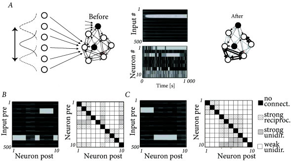
The results of simulations of the Clopath model shown in Fig. 19.10 can be interpreted as a realization of a soft form of competitive learning. Neurons form subnetworks that specialize on the same features of the input. Because of inhibition, different subnetworks specialize on different segments of the input space.

Ten excitatory neurons (with all-to-all connectivity) are linked to three inhibitory neurons. Each inhibitory neuron receives input from 8 randomly selected excitatory neurons and randomly projects back to 6 excitatory neurons ( 99 ) . In addition to the recurrent input, each excitatory and inhibitory neuron receives feedforward spike input from 500 presynaptic neurons $j$ that generate stochastic Poisson input at a rate $\nu_{j}$ . The input neurons can be interpreted as a sensory array. The rates of neighboring input neurons are correlated, mimicking the presence of a spatially extended object stimulating the sensory layer. Spiking rates at the sensory layer change every 100ms.

Feedforward connections and lateral connections between model pyramidal neurons are plastic whereas connections to and from inhibitory neurons are fixed. In a simulation of the model network, the excitatory neurons developed localized receptive fields, i.e., weights from neighboring inputs to the same postsynaptic neuron become either strong or weak together (Fig. 19.10 A). Similarly, lateral connections onto the same postsynaptic neuron develop strong or weak synapses, that remain, apart from fluctuations, stable thereafter (Fig. 19.10 A) leading to a structured pattern of synaptic connections (Fig. 19.10 B). While the labeling of the excitatory neurons at the beginning of the experiment was randomly assigned, we can relabel the neurons after the formation of lateral connectivity patterns so that neurons with similar receptive fields have similar indices. After reordering we can clearly distinguish that two groups of neurons have been formed, characterized by similar receptive fields and strong bidirectional connectivity within the group, and different receptive fields and no lateral connectivity between groups (Fig. 19.10 C).

Fig. 19.10: Receptive field development and lateral connectivity. A. A network of 10 excitatory neurons (empty circles, not all neurons are shown) is connected to 3 inhibitory neurons (filled circle) and receives feedforward inputs from 500 Poisson spike trains with a Gaussian profile of firing rates. The center of the Gaussian is shifted randomly every 100ms. Between the two schematic figures represeting the network before (left) and after the plasticity experiment (right), we depict the evolution of input weights and recurrent excitatory weights onto one selected excitatory neuron. B Mean feedforward weights (left) and recurrent excitatory weights (right) averaged over 100s. The gray level graph for the feedforward weights (left) indicates that neurons develop receptive fields that are localized in the input space. The diagonal in the matrix of recurrent connectivity is black, since self-connections do not exist in the model. C. Same as (B) but for the sake of visual clarity the index of neurons is reordered so that neurons with similar receptive fields have adjacent numbers, highlighting that neurons with similar receptive fields (e.g., neurons 1 to 3) have strong bilateral connections. Adapted from Clopath et al. (99).

19.3.2 Learning equations for rate models

We focus on a single analog neuron that receives input from $N$ presynaptic neurons with firing rates $\nu_{j}^{\text{pre}}$ via synapses with weights $w_{j}$ ; cf. Fig. 19.11 A. Note that we have dropped the index $i$ of the postsynaptic neuron since we focus in this section on a single output neuron. We think of the presynaptic neurons as ‘input neurons’, which, however, do not have to be sensory neurons. The input layer could, for example, may consist of neurons in the lateral geniculate nucleus (LGN) that project to neurons in the visual cortex. As before, the firing rate of the input neurons is modeled by the static pattern scenario. We will show that the statistical properties of the input control the evolution of synaptic weights. In particular, we identify the conditions under which unsupervised Hebbian learning is related to Principal Component Analysis (PCA).

In the following we analyze the evolution of synaptic weights using the simple Hebbian learning rule of Eq. ( 19.3 ). The presynaptic activity drives the postsynaptic neuron and the joint activity of pre- and postsynaptic neurons triggers changes of the synaptic weights:

\Delta w_{i}=\gamma\,\nu^{\text{post}}\,\nu_{i}^{\text{pre}}\,.

(19.21)

Here, $0<\gamma\ll 1$ is a small constant called ‘learning rate’. The learning rate in the static-pattern scenario is closely linked to the correlation coefficient $c^{\text{corr}}_{11}$ in the continuous-time Hebb rule introduced in Eq. ( 19.3 ). In order to highlight the relation, let us assume that each pattern $\mbox{\boldmath$\xi$}^{\mu}$ is applied during an interval $\Delta t$ . For $\Delta t$ sufficiently small, we have $\gamma=c^{\text{corr}}_{11}\,\Delta t$ .

Fig. 19.11: Elementary model. A. Patterns $\mbox{\boldmath$\xi$}^{\mu}$ are applied as a set of presynaptic firing rates $\nu_{j}$ , i.e., $\mbox{\boldmath$\xi$}^{\mu}_{j}=\nu_{j}^{\rm pre}$ for $1\leq j\leq N$ . B. The gain function of the postsynaptic neuron is taken as linear, i.e., $\nu^{\rm post}=h$ . It can be seen as a linearization of the sigmoidal gain function $g(h)$ .

In a general rate model, the firing rate $\nu^{\text{post}}$ of the postsynaptic neuron is given by a nonlinear function of the total input

\nu^{\text{post}}=g\left(\sum_{j}w_{j}\,\nu_{j}^{\text{pre}}\right)\,\,;

(19.22)

cf. Fig. 19.11 B and Chapter 15 . For the sake of simplicity, we restrict our discussion in the following to a linear rate model with

\nu^{\text{post}}=\sum_{j}w_{j}\,\nu_{j}^{\text{pre}}={\bf w}\cdot{\mbox{% \boldmath\(\nu\)}}^{\text{pre}}\,,

(19.23)

where we have introduced a vector notation for the weights ${\bf w}=(w_{1},\dots,w_{N})$ , the presynaptic rates ${\mbox{\boldmath$\nu$}}^{\text{pre}}=(\nu_{1},\dots\nu_{N})$ and the dot denotes a scalar product. Hence we can interpret the output rate $\nu^{\text{post}}$ as a projection of the input vector onto the weight vector.

If we combine the learning rule ( 19.21 ) with the linear rate model of Eq. ( 19.23 ) we find after the presentation of pattern $\mbox{\boldmath$\xi$}^{\mu}$

\Delta w_{i}=\gamma\,\sum_{j}w_{j}\,\nu_{j}^{\text{pre}}\,\nu_{i}^{\text{pre}}% =\gamma\,\sum_{j}w_{j}\,\xi^{\mu}_{j}\,\xi^{\mu}_{i}\,.

(19.24)

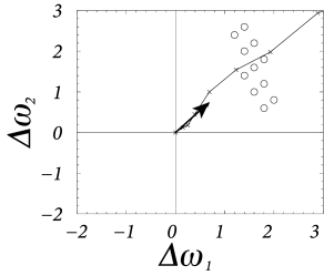
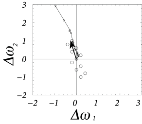
The evolution of the weight vector $\mbox{\boldmath$w$}=(w_{1},\ldots,w_{N})$ is thus determined by the iteration

w_{i}(n+1)=w_{i}(n)+\gamma\,\sum_{j}w_{j}\,\xi^{\mu_{n}}_{j}\,\xi^{\mu_{n}}_{i% }\,,

(19.25)

where $\mu_{n}$ denotes the pattern that is presented during the $n$ th time step. Eq. ( 19.25 ) is called an ‘online’ rule, because the weight update happens immediately after the presentation of each pattern. The evolution of the weight vector ${\bf w}=(w_{1},\dots,w_{N})$ during the presentation of several patterns is shown in Fig. 19.12 .

Fig. 19.12: Weight changes induced by the standard Hebb rule. Input patterns $\mbox{\boldmath$\xi$}^{\mu}\in\mathbb{R}^{2}$ are marked as circles. The sequence of weight vectors $\mbox{\boldmath$w$}(1)$ , $\mbox{\boldmath$w$}(2)$ , …, is indicated by crosses connected by a solid line. A. The weight vector evolves in direction of the center of mass of the cloud of data points, because this is the dominant eigenvector of the (non-normalized) correlation matrix of the data. B. If the input patterns are normalized so that their center of mass is at the origin, then the weight vector becomes parallel to the first principal component $\mbox{\boldmath$e$}_{1}$ of the data set.

If the learning rate $\gamma$ is small, a large number of patterns has to be presented in order to induce a substantial weight change. In this case, there are two equivalent routes to proceed with the analysis. The first one is to study a version of learning where all $P$ patterns are presented before an update occurs. Thus, Eq. ( 19.25 ) is replaced by

w_{i}(n+1)=w_{i}(n)+\tilde{\gamma}\,\sum_{j}w_{j}\,\sum_{\mu=1}^{P}\xi^{\mu}_{% j}\,\xi^{\mu}_{i}\,

(19.26)

with a new learning rate $\tilde{\gamma}=\gamma/P$ . This is called a ‘batch update’. With the batch update rule, the right hand side can be rewritten as

w_{i}(n+1)=w_{i}(n)+\gamma\,\sum_{j}C_{ij}\,w_{j}(n)\,,\,

(19.27)

where we have introduced the correlation matrix

C_{ij}=\frac{1}{P}\sum_{\mu=1}^{P}\xi_{i}^{\mu}\,\xi_{j}^{\mu}=\langle\xi_{i}^% {\mu}\,\xi_{j}^{\mu}\rangle_{\mu}\,.

(19.28)

Thus, the evolution of the weights is driven by the correlations in the input.

The second, alternative, route is to stick to the online update rule, but study the expectation value of the weight vector, i.e., the weight vector $\left<\mbox{\boldmath$w$}(n)\right>$ averaged over the sequence $(\mbox{\boldmath$\xi$}^{\mu_{1}},\mbox{\boldmath$\xi$}^{\mu_{2}},\dots,% \mbox{\boldmath$\xi$}^{\mu_{n}})$ of all patterns that so far have been presented to the network. From Eq. ( 19.25 ) we find

$\displaystyle\left<w_{i}(n+1)\right>$	$\displaystyle=\left<w_{i}(n)\right>+\gamma\,\sum_{j}\left<w_{j}(n)\,\xi^{\mu_{% n+1}}_{j}\,\xi^{\mu_{n+1}}_{i}\right>$
	$\displaystyle=\left<w_{i}(n)\right>+\gamma\,\sum_{j}\left<w_{j}(n)\right>\,% \left<\xi^{\mu_{n+1}}_{j}\,\xi^{\mu_{n+1}}_{i}\right>$
	$\displaystyle=\left<w_{i}(n)\right>+\gamma\,\sum_{j}C_{ij}\,\left<w_{j}(n)% \right>\,.$	(19.29)

The angular brackets denote an ensemble average over the whole sequence of input patterns $(\mbox{\boldmath$\xi$}^{\mu_{1}},\mbox{\boldmath$\xi$}^{\mu_{2}},\dots)$ . The second equality is due to the fact that input patterns are chosen independently in each time step, so that the average over $w_{j}(n)$ and $(\xi^{\mu_{n+1}}_{j}\,\xi^{\mu_{n+1}}_{i})$ can be factorized. Note that Eq. ( 19.3.2 ) for the expected weights in the online rule is equivalent to Eq. ( 19.27 ) for the weights in the batch rule.

Expression ( 19.3.2 ), or equivalently ( 19.27 ), can be written in a more compact form using matrix notation (we drop the angular brackets in the following)

\mbox{\boldmath\(w\)}(n+1)=({\bf 1\hskip{-2.8pt}I}+\gamma\,C)\,\mbox{\boldmath% \(w\)}(n)=({\bf 1\hskip{-2.8pt}I}+\gamma\,C)^{n+1}\,\mbox{\boldmath\(w\)}(0)\,,

(19.30)

where $\mbox{\boldmath$w$}(n)=\left(w_{1}(n),\ldots,w_{N}(n)\right)$ is the weight vector and ${\bf 1\hskip{-2.8pt}I}$ is the identity matrix.

If we express the weight vector in terms of the eigenvectors $\mbox{\boldmath$e$}_{k}$ of $C$ ,

\mbox{\boldmath\(w\)}(n)=\sum_{k}a_{k}(n)\,\mbox{\boldmath\(e\)}_{k}\,,

(19.31)

we obtain an explicit expression for $\mbox{\boldmath$w$}(n)$ for any given initial condition $a_{k}(0)$ , viz.,

\mbox{\boldmath\(w\)}(n)=\sum_{k}(1+\lambda_{k})^{n}\,a_{k}(0)\,\mbox{% \boldmath\(e\)}_{k}\,.

(19.32)

Since the correlation matrix is positive semi-definite, all eigenvalues $\lambda_{k}$ are real and positive. Therefore, the weight vector is growing exponentially, but the growth will soon be dominated by the eigenvector with the largest eigenvalue, i.e., the first principal component ,

\mbox{\boldmath\(w\)}(n)\xrightarrow{n\to\infty}(1+\lambda_{1})^{n}\,a_{1}(0)% \,\mbox{\boldmath\(e\)}_{1}\,.

(19.33)

Recall that the output of the linear neuron model ( 19.23 ) is proportional to the projection of the current input pattern $\mbox{\boldmath$\xi$}^{\mu}$ on the direction $w$ . For $\mbox{\boldmath$w$}\propto\mbox{\boldmath$e$}_{1}$ , the output is therefore proportional to the projection on the first principal component of the input distribution. A Hebbian learning rule such as ( 19.21 ) is thus able to extract the first principal component of the input data.

From a data-processing point of view, the extraction of the first principal component of the input data set by a biologically inspired learning rule seems to be very compelling. There are, however, a few drawbacks and pitfalls when using the above simple Hebbian learning scheme. Interestingly, all three can be overcome by slight modifications in the Hebb rule.

First, the above statement about the Hebbian learning rule is limited to the expectation value of the weight vector. However, it can be shown that if the learning rate is sufficiently low, then the actual weight vector is very close to the expected one so that this is not a major limitation.

Second, while the direction of the weight vector moves in the direction of the principal component, the norm of the weight vector grows without bounds. However, variants of Hebbian learning such as the Oja learning rule ( 19.7 ) allow us to normalize the length of the weight vector without changing its direction; cf. Exercises.

Third, principal components are only meaningful if the input data is normalized, i.e., distributed around the origin. This requirement is not consistent with a rate interpretation because rates are usually positive. This problem, however, can be overcome by learning rules such as the covariance rule of Eq. ( 19.6 ) that are based on the deviation of the rates from a certain mean firing rate. Similarly, STDP rules can be designed in a way that the output rate remains normalized so that learning is sensitive only to deviations from the mean firing rate and can thus find the first principal component even if the input is not properly normalized ( 256; 489; 257 ) .

Example: Correlation matrix and Principal Component Analysis

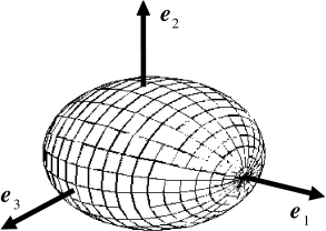
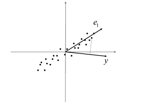
For readers not familiar with principal component analysis (PCA) we review here the basic ideas and main results. PCA is a standard technique to describe statistical properties of a set of high-dimensional data points and is performed to find the direction in which the data shows the largest variance. If we think of the input data set as of a cloud of points in a high-dimensional vector space centered around the origin, then the first principal component is the direction of the longest axis of the ellipsoid that encompasses the cloud; cf. Fig. 19.13 A. In the following, we will explain the basic idea and show that the first principal component gives the direction where the variance of the data is maximal.

Let us consider an ensemble of data points $\{\mbox{\boldmath$\xi$}^{1},\dots,\mbox{\boldmath$\xi$}^{P}\}$ drawn from a (high-dimensional) vector space, for example $\mbox{\boldmath$\xi$}^{\mu}\in\mathbb{R}^{N}$ . For this set of data points we define the correlation matrix $C_{ij}$ as

C_{ij}=\frac{1}{P}\sum_{\mu=1}^{P}\xi_{i}^{\mu}\,\xi_{j}^{\mu}=\left<\xi_{i}^{% \mu}\,\xi_{j}^{\mu}\right>_{\mu}\,.

(19.34)

Angular brackets $\left<\cdot\right>_{\mu}$ denote an average over the whole set of data points. Similar to the variance of a single random variable we can also define the covariance matrix $V_{ij}$ of our data set,

V_{ij}=\left<(\xi_{i}^{\mu}-\langle\xi_{i}^{\mu}\rangle_{\mu})\,(\xi_{j}^{\mu}% -\langle\xi_{j}^{\mu}\rangle_{\mu})\right>_{\mu}\,.

(19.35)

In the following we will assume that the coordinate system is chosen so that the center of mass of the set of data points is located at the origin, i.e., $\left<\xi_{i}\right>_{\mu}=\left<\xi_{j}\right>_{\mu}=0$ . In this case, correlation matrix and covariance matrix are identical.

The principal components of the set $\{\mbox{\boldmath$\xi$}^{1},\dots,\mbox{\boldmath$\xi$}^{P}\}$ are defined as the eigenvectors of the covariance matrix $V$ . Note that $V$ is symmetric, i.e., $V_{ij}=V_{ji}$ . The eigenvalues of $V$ are thus real-valued and different eigenvectors are orthogonal ( 229 ) . Furthermore, $V$ is positive semi-definite since

y

(19.36)

for any vector $\mbox{\boldmath$y$}\in\mathbb{R}^{N}$ . Therefore, all eigenvalues of $V$ are non-negative.

We can sort the eigenvectors $\mbox{\boldmath$e$}_{i}$ according to the size of the corresponding eigenvalues $\lambda_{1}\geq\lambda_{2}\geq\dots\geq 0$ . The eigenvector with the largest eigenvalue is called the first principal component.

The first principal component points in the direction where the variance of the data is maximal. To see this we calculate the variance of the projection of $\mbox{\boldmath$\xi$}^{\mu}$ onto an arbitrary direction $y$ (Fig. 19.13 B) that we write as $\mbox{\boldmath$y$}=\sum_{i}a_{i}\,\mbox{\boldmath$e$}_{i}$ with $\sum_{i}a_{i}^{2}=1$ so that $\|\mbox{\boldmath$y$}\|=1$ . The variance $\sigma^{2}_{\mbox{\boldmath$y$}}$ along $y$ is

\sigma^{2}_{\mbox{\boldmath\(y\)}}=\left<\left[\mbox{\boldmath\(\xi\)}^{\mu}% \cdot\mbox{\boldmath\(y\)}\right]^{2}\right>_{\mu}=\mbox{\boldmath\(y\)}^{% \text{T}}\,V\,\mbox{\boldmath\(y\)}=\sum_{i}\lambda_{i}\,a_{i}^{2}\,.

(19.37)

The right-hand side is maximal under the constraint $\sum_{i}a_{i}^{2}=1$ if $a_{1}=1$ and $a_{i}=0$ for $i=2,3,\dots,N$ , that is, if $\mbox{\boldmath$y$}=\mbox{\boldmath$e$}_{1}$ .

Fig. 19.13: Principal Component Analysis. A. Ellipsoid approximating the shape of a cloud of data points. The first principal component $\mbox{\boldmath$e$}_{1}$ corresponds to the principal axis of the ellipsoid. B. Sample distribution of data points in two dimensions. The first principal component $\mbox{\boldmath$e$}_{1}$ points in the direction where the variance of the data is maximal. Projection (dashed line) of data points onto an arbitrary other axis $y$ gives a distribution of smaller variance.

19.3.3 Learning equations for STDP models (*)

The evolution of synaptic weights in the pair-based STDP model of Eq. ( 19.10 ) can be assessed by assuming that pre- and postsynaptic spike trains can be described by Poisson processes. For the postsynaptic neuron, we take the linear Poisson model in which the output spike train is generated by an inhomogeneous Poisson process with rate

\nu_{i}(u_{i})=\left[\alpha\,u_{i}-\nu_{0}\right]_{+}

(19.38)

with scaling factor $\alpha$ , threshold $\nu_{0}$ and membrane potential $u_{i}(t)=\sum_{j}w_{ij}\epsilon\left(t-t_{j}^{f}\right)$ , where $\epsilon(t)$ denotes the time course of an excitatory postsynaptic potential generated by a presynaptic spike arrival. The notation $[x]_{+}$ denotes a piecewise linear function: $[x]_{+}=x$ for $x>0$ and zero otherwise. In the following we assume that the argument of our piecewise linear function is positive so that we can suppress the square brackets.

For the sake of simplicity, we assume that all input spike trains are Poisson processes with a constant firing rate $\nu_{j}$ . In this case the expected firing rate of the postsynaptic neuron is simply:

\langle\nu_{i}\rangle=-\nu_{0}+\alpha\bar{\epsilon}\sum_{j}w_{ij}\,\nu_{j}\,,

(19.39)

where $\bar{\epsilon}=\int\epsilon(s){\text{d}}s$ is the total area under an excitatory postsynaptic potential. The conditional rate of firing of the postsynaptic neuron, given an input spike at time $t_{j}^{f}$ is given by

\nu_{i}(t)=-\nu_{0}+\alpha\bar{\epsilon}\sum_{j}w_{ij}\nu_{j}+\alpha w_{ij}% \epsilon\left(t-t_{j}^{f}\right)\,.

(19.40)

Since the conditional rate is different from the expected rate, the postsynaptic spike train $S_{i}(t)$ is correlated with the presynaptic spike trains $S_{j}(t^{\prime})$ . The correlations can be calculated to be

\Gamma_{ji}(s)=\langle S_{i}(t+s)S_{j}(t)\rangle=\langle\nu_{i}\rangle\nu_{j}+% \alpha\,w_{ij}\nu_{j}\,\epsilon(s)\,.

(19.41)

Similar to the expected weight evolution for rate models in Section 19.3.2 , we now study the expected weight evolution in the spiking model with the pair-based plasticity rule of Eq. 19.10 . The result is ( 256 )

\langle\dot{w_{ij}}\rangle={\nu}_{j}\,\langle\nu_{i}\rangle\,[-A_{-}(w_{ij})% \tau_{-}+A_{+}\left(w_{ij}\right)\tau_{+}]+\alpha w_{ij}\nu_{j}\,A_{+}(w_{ij})% \int W_{+}(s)\epsilon(s){\text{d}}s\>.

(19.42)

The first term is reminiscent of rate-based Hebbian learning, Eq. ( 19.3 ), with a coefficient $c^{\text{corr}}_{11}$ proportional to the integral under the learning window. The last term is due to pre-before-post spike timings that are absent in a pure rate model. Hence, despite the fact that we started off with a pair-based STDP rule, the synaptic dynamics contains a term of the form $\alpha\nu_{j}w\,A_{+}(w)\int W_{+}(s)\epsilon(s){\text{d}}s$ that is linear in the presynaptic firing rate ( 256; 257 ) .

Example: Stabilization of postsynaptic firing rate

If spike arrival rates $\nu_{j}=\nu$ at all synapses are identical, we expect a solution of the learning equation to exist where all weights are identical, $w_{ij}=w$ . For simplicity we drop the averaging signs. Eq. ( 19.42 ) then becomes

\frac{\dot{w}}{\nu}=\nu_{i}\,[-A_{-}(w)\tau_{-}+A_{+}\left(w\right)\tau_{+}]+% \alpha wA_{+}(w)\int W_{+}(s)\epsilon(s){\text{d}}s\>.

(19.43)

Moreover, we can use Eq. ( 19.39 ) to express the postsynaptic firing rate in terms of the input rate $\nu$ .

\nu_{i}=-\nu_{0}+\alpha\nu\bar{\epsilon}N\,w\,.

(19.44)

If the weight $w$ increases, the postsynaptic firing rate does as well. We now ask whether the postsynaptic firing has a fixed point $\nu_{FP}$ .

The fixed point analysis can be performed for a broad class of STDP models. However, for the sake of simplicity we focus on the model with hard bounds in the range where $0<w<w^{\rm max}$ . We introduce a constant $C=A_{-}(w)\tau_{-}-A_{+}\left(w\right)\tau_{+}$ . If the integral of the learning window is negative, then $C>0$ and LTD dominates over LTP. In this case, a fixed point exists at

\nu_{\mathrm{FP}}=\frac{C_{\mathrm{ss}}\nu_{0}}{NC\nu\bar{\epsilon}-C_{\mathrm% {ss}}}

(19.45)

where $C_{\mathrm{ss}}=A_{+}(w)\int W_{+}(s)\epsilon(s){\text{d}}s$ denotes the contribution of the spike-spike correlations. The mean firing rate of the neuron is, under rather general conditions, stabilized at the fixed point ( 257 ) . Hence STDP can lead to a control of the postsynaptic firing rate ( 256; 489; 257 ) . We emphasize that the existence of a fixed point and its stability does not crucially depend on the presence of soft or hard bounds on the weights. Since for constant input rates $\nu$ , we have $\nu_{i}=\nu_{0}+\alpha\nu\bar{\epsilon}\sum_{j}w_{ij}$ , stabilization of the output rate automatically implies normalization of the summed weights.