20.1 Reservoir computing
One of the reasons, the dynamics of neuronal networks are rich is that networks have a non-trivial connectivity structure linking different neuron types in an intricate interaction pattern. Moreover, network dynamics are rich because they span many time scales. The fastest time scale is set by the duration of an action potential, i.e. a few milliseconds. Synaptic facilitation and depression (Ch. 3 ) or adaptation (Ch. 6 ) occur on the time scales from a few hundred milliseconds to seconds. Finally, long-lasting changes of synapses can be induced in a few seconds, but last from hours to days (Ch. 19 ). Moreover,
These rich dynamics of neuronal networks can be used as a ‘reservoir’ for intermediate storage and representation of incoming input signals. Desired outputs can then be constructed by reading out appropriate combinations of neuronal spike trains from the network. This kind of ‘reservoir computing’ encompasses the notions of ‘liquid computing’ ( 313 ) and ’echo state networks’ ( 241 ) . Before we discuss some mathematical aspects of randomly connected networks, we illustrate rich dynamics by a simulated model network.
20.1.1 Rich dynamics
A nice example of rich network dynamics is work by Maass et al. 2007. Six hundred leaky integrate-and-fire neurons (80 percent excitatory and 20 percent inhibitory) were placed on a three-dimensional grid with distance-dependent random connectivity of small probability so that the total number of synapses is about 10’000. Synaptic dynamics included short-term plasticity (Ch. 3 ) with time constants ranging from a few tens of milliseconds to a few seconds. Neuronal parameters varied from one neuron to the next and each neuron received independent noise.
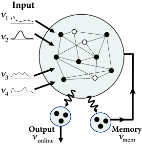
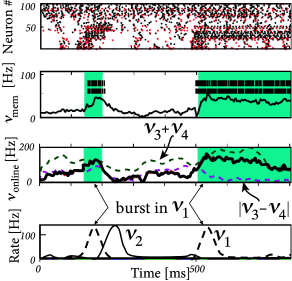
In order to check the computational capabilities of such a network, Maass et al. stimulated it with four input streams targeting different subgroups of the network (Fig. 20.1 ). Each input stream consisted of Poisson spike trains with time-dependent firing rate .
Streams one and two fired at a low background rate but switched occasionally to a short period of high firing rate (’burst’). In order to build a memory of past bursts, synaptic weights from the network onto a group of eight integrate-and-fire neurons (‘memory’ in Fig. 20.1 ) were adjusted by some optimization algorithm, so that the spiking activity of these eight neurons reflects whether the last firing-rate burst happened in stream one (memory neurons are active = memory ‘on’) or two (the same neurons are inactive = memory ‘off’). Thus, these neurons provided a 1-bit memory (’on’/’off’) of past events.
Streams three and four were used to perform a non-trivial online computation. A network output with value was optimized to calculate the sum of activity in streams three and four, but only if the memory neurons were active (memory ’on’). Optimization of weight parameters was achieved, in a series of preliminary training trials by minimizing the squared error (Ch. 10 ) between the target and the actual output.
Figure 20.1 shows that, after optimization of the weights, the network could store a memory and, at the same time, perform the desired online computation. Therefore, the dynamics in a randomly connected network with feedback from the output are rich enough to generate an output stream which is a non-trivial nonlinear transformation of the input streams ( 312; 241; 502 ) .
| A | B |
|---|---|
|
|
In the above simulation, the tunable connections (Fig. 20.1 A) have been adjusted ‘by hand’ (or rather by a suitable algorithm), in a biologically non-plausible fashion, so as to yield the desired output. However, it is possible to learn the desired output with the three-factor learning rules discussed in Section 19.4 of Ch. 19 . This has been demonstrated on a task and set-up very similar to Fig. 20.1 , except that the neurons in the network were modeled by rate units ( 225 ) . The neuromodulatory signal (cf. Section 19.4 ) took a value of one, if the momentary performance was better than the average performance in the recent past, and zero otherwise.
20.1.2 Network analysis (*)
Networks of randomly connected excitatory and inhibitory neurons can be analyzed for the case of rate units ( 413 ) . Let denote the deviation from a spontaneous background rate , i.e., the rate of neuron is . Let us consider the update dynamics
| (20.1) |
for a monotone transfer function with and derivative .
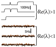
The background state ( for all neurons ) is stable if the weight matrix has no eigenvalues with real part larger than one. If there are eigenvalues with real part larger than one, spontaneous chaotic network activity may occur ( 487 ) .
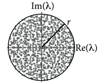
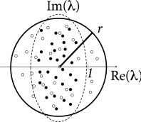
For weight matrices of random networks, a surprising number of mathematical results exists. We focus on mixed networks of excitatory and inhibitory neurons. In a network of neurons, there are excitatory and inhibitory neurons where is the fraction of excitatory neurons. Outgoing weights from an excitatory neuron take values for all , (and for weights from inhibitory neurons), so that all columns of the weight matrix have the same sign. We assume non-plastic random weights with the following three constraints: (i) Input to each neuron is balanced so that for all (‘detailed balance’). In other words, if all neurons are equally active, excitation and inhibition cancel each other on a neuron-by-neuron level. (ii) Excitatory weights are drawn from a distribution with mean and variance . (iii) Inhibitory weights are drawn from a distribution with mean and variance . Under the conditions (i) - (iii), the eigenvalues of the weight matrix all lie within a circle (Fig. 20.2 A) of radius , called the spectral radius ( 413 ) .
| A | B | C |
|---|---|---|
|
|
|
The condition of detailed balance stated above as item (i) may look artificial at first sight. However, experimental data supports the idea of detailed balance ( 161; 370 ) . Moreover, plasticity of inhibitory synapses can be used to achieve such a balance of excitation and inhibition on a neuron-by-neuron basis ( 539 ) .
To understand how inhibitory plasticity comes into play, consider a rate model in continuous time
| (20.2) |
where is a time constant and is, as before, the deviation of the firing rate from a background level . The gain function with and is bounded between and . Gaussian white noise of small amplitude is added on the right-hand side of Eq. ( 20.2 ) so as to kick network activity out of the fixed point at .
We subject inhibitory weights (where is one of the inhibitory neurons) to Hebbian plasticity
| (20.3) |
where is the synaptic trace left by earlier presynaptic activity. For , this is a Hebbian learning rule because the absolute size of the inhibitory weight increases, if postsynaptic and presynaptic activity are correlated (Ch. 19 ).
In a random network of excitatory and inhibitory rate neurons with an initial weight matrix that had a large distribution of eigenvalues, inhibitory plasticity according to Eq. ( 20.3 ) led to a compression of the real parts of the eigenvalues ( 213 ) . Hebbian inhibitory plasticity can therefore push a network from the regime of unstable dynamics into a stable regime (Fig. 20.2 B,C) while keeping the excitatory weights strong. Such networks, which have strong excitatory connections, counterbalanced by equally strong precisely tuned inhibition, can potentially explain patterns of neural activity in motor cortex during arm movements ( 98 ) . In depth understanding of patterns in motor cortex could eventually contribute to the development of neural prosthesis ( 472 ) that detect and decode neural activity in motor-related brain areas and translate it into intended movements of a prosthetic limb; cf. Chapter 11 .
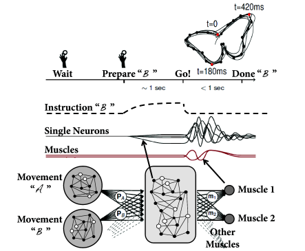
Example: Generating movement trajectories with inhibition stabilized networks
During the preparation and performance of arm movements (Fig. 20.3 A) neurons in motor cortex exhibit collective dynamics ( 98 ) . In particular, during the preparation phase just before the start of the movement, the network activity approaches a stable pattern of firing rates, which is similar across different trials. This stable pattern can be interpreted as an initial condition for the subsequent evolution of the network dynamics during arm movement which is rather stereotypical across trials ( 472 ) .
Because of its sensitivity to small perturbations, a random network with chaotic network dynamics may not be a plausible candidate for stereotypical dynamics, necessary for reliable arm movements. On the other hand, in a stable random network with a circular distribution of eigenvalues with spectral radius , transient dynamics after release from an initial condition are short and dominated by the time constant of the single-neuron dynamics (unless one of the eigenvalues is hand-tuned to lie very close to unity). Moreover, as discussed in Ch. 18 , cortex is likely to work in the regime of an inhibition-stabilized network ( 524; 374 ) where excitatory connections are strong, but counterbalanced by even stronger inhibition.
Inhibitory plasticity is helpful to generate inhibition stabilized random networks. Because excitatory connections are strong but random, transient activity after release from an appropriate initial condition is several times longer than the single-neuron time constant . Different initial conditions put the network onto different, but reliable trajectories. These trajectories of the collective network dynamics can be used as a reservoir to generate simulated muscle output for different arm trajectories (Fig. 20.3 ).