20 Outlook: Dynamics in Plastic Networks 20.1 Reservoir computing 20.3 Helping Patients

20.2 Oscillations: good or bad?

Oscillations are a prevalent phenomenon in biological neural systems and manifest themselves experimentally in electroencephalograms (EEG), recordings of local field potentials (LFP), and multi-unit recordings. Oscillations are thought to stem from synchronous network activity and are often characterized by the associated frequency peak in the Fourier spectrum. For example, oscillations in the range of 30-70Hz are called gamma-oscillations and those above 100Hz ‘ultrafast’ or ‘ripples’ ( 518; 85 ) . Among the slower oscillations, prominent examples are delta oscillations (1-4Hz) and spindle oscillations in the EEG during sleep (7-15Hz) ( 42 ) or theta oscillations (4-10Hz) in hippocampus and other areas ( 85 ) .

Oscillations are thought to play an important role in the coding of sensory information. In the olfactory system an ongoing oscillation of the population activity provides a temporal frame of reference for neurons coding information about the odorant ( 292 ) . Similarly, place cells in the hippocampus exhibit phase-dependent firing activity relative to a background oscillation ( 375; 85 ) . Moreover, rhythmic spike patterns in the inferior olive may be involved in various timing tasks and motor coordination ( 548; 261 ) . Finally, synchronization of firing across groups of neurons has been hypothesized to provide a potential solution to the so-called binding problem ( 479; 480 ) . The common idea across all the above examples is that an oscillation provides a reference signal for a ‘phase code’: the significance of a spike depends on its phase with respect to the global oscillatory reference; cf. Sect. 7.6 and Fig. 7.17 in Ch. 7 . Thus, oscillations are potentially useful for intricate neural coding schemes.

On the other hand, synchronous oscillatory brain activity is correlated with numerous brain diseases. For example, an epileptic seizure is defined as ’a transient occurrence of signs and/or symptoms due to abnormal excessive or synchronous neuronal activity in the brain’ ( 150 ) . Similarly, Parkinson’s disease is characterized by a high level of neuronal synchrony in the thalamus and basal ganglia ( 387 ) while neurons in the same areas fire asynchronously in the healthy brain ( 366 ) . Moreover, local field potential oscillations at theta frequency in thalamic or subthalamic nuclei is linked to tremor in human Parkinsonian patients, i.e. rhythmic finger, hand or arm movement at 3-6Hz ( 387; 504 ) . Therefore, in these and in similar situations, it seems to be desirable to suppress abnormal, highly synchronous oscillations so as to shift the brain back into its healthy state.

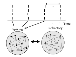
Simulations of the population activity in homogeneous networks typically exhibit oscillations when driven by a constant external input. For example, oscillations in networks of purely excitatory neurons arise because, as soon as some neurons in the network fire they contribute to exciting others. Once the avalanche of firing has run across the network, all neurons pass through a period of refractoriness, until they are ready to fire again. In this case the time scale of the oscillation is set by neuronal refractoriness (Fig. 20.4 A). A similar argument can be made for a homogeneous network of inhibitory neurons driven by a constant external stimulus. After a first burst by a few neurons, mutual inhibition will silence the population until inhibition wears off. Thereafter, the whole network fires again.

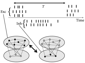
Oscillations also arise in networks of coupled excitatory and inhibitory neurons. The excitatory connections cause a synchronous bursts of the network activity leading to a build-up of inhibition which, in turn, suppresses the activity of excitatory neurons. The oscillation period in the two latter cases is therefore set by the build-up and decay time of inhibitory feedback (Fig. 20.4 B).

Even slower oscillations can be generated in ‘winner-take-all’ networks (cf. Chapter 16 ) with dynamic synapses (cf. Chapter 3 ) or adaptation (cf. Chapter 6 ). Suppose the networks consists of $K$ populations of excitatory neurons which share a common pool of inhibitory neurons. Parameters can be set such that excitatory neurons within the momentarily ‘winning’ population stimulate each other so as to overcome inhibition. In the presence of synaptic depression, however, the mutual excitation fades away after a short time, so that now a different excitatory population becomes the new ‘winner’ and switches on. As a result, inhibition arising from inhibitory neurons turns the activity of the previously winning group off, until inhibition has decayed and excitatory synapses have recovered from depression. The time scale is then set by combination of the time scales of inhibition and synaptic depression. Networks of this type have been used to explain the shift of attention from one point in a visual scene to the next ( 236 ) .

Fig. 20.4: Types of network oscillation. A. In a homogeneous network of excitatory neurons, near-synchronous firing of all neurons is followed by a period of refractoriness, leading to fast oscillations with period $T$ . Active neurons: vertical dash in spike raster and filled circle in network schema. Silent neurons: open circle in schema. B. In a network of excitatory and inhibitory neurons, activity of the excitatory population alternates with activity of inhibitory one. The period $T$ is longer than in A.

In this section, we briefly review mathematical theories of oscillatory activity (subsections 20.2.1 - 20.2.3 ) before we study the interaction of oscillations with STDP (subsection 20.2.4 ) The results of this section will form the basis for the discussion of Section 20.3 .

20.2.1 Synchronous Oscillations and Locking

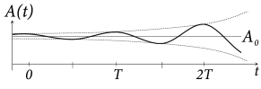
Homogeneous networks of spiking neurons show a natural tendency toward oscillatory activity. In Sections 13.4.2 and 14.2.3 , we have analyzed the stability of asynchronous firing. In the stationary state the population activity is characterized by a constant value $A_{0}$ of the population activity. An instability of the dynamics with respect to oscillations at period $T$ , appears as a sinusoidal perturbation of increasing amplitude; see Fig. 20.5 A as well as Fig. 14.8 in Ch. 14 . The analysis of the stationary state shows that a high level of noise, network heterogeneity, or a sufficient amount of inhibitory plasticity all contribute to stabilizing the stationary state. The linear stability analysis, however, is only valid in the vicinity of the stationary state. As soon as the amplitude $\Delta A$ of the oscillations is of the same order of magnitude as $A_{0}$ , the solution found by linear analysis is no longer valid since the population activity cannot become negative.

Oscillations can, however, also be analyzed from a completely different perspective. In a homogeneous network with fixed connectivity in the limit of low noise we expect strong oscillations. In the following, we focus on the synchronous oscillatory mode where nearly all neurons fire in ‘lockstep’ (Fig. 20.5 B). We study whether such periodic synchronous burst of the population activity can be a stable solution of network equations.

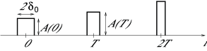
To keep the arguments simple, we consider a homogeneous population of identical SRM ${}_{0}$ neurons (Ch. 6 and Sect. 9.3 in Ch. 9 ) which is nearly perfectly synchronized and fires almost regularly with period $T$ . In order to analyze the existence and stability of a fully locked synchronous oscillation we approximate the population activity by a sequence of square pulses $k$ , $k\in\{0,\pm 1,\pm 2,\ldots\}$ , centered around $t=k\,T$ . Each pulse $k$ has a certain half-width $\delta_{k}$ and amplitude $(2\delta_{k})^{-1}$ – since all neurons are supposed to fire once in each pulse; cf. Fig. 20.5 B. If we find that the amplitude of subsequent pulses increases while their width decreases (i.e., $\lim_{k\to\infty}\delta_{k}=0$ ), we conclude that the fully locked state in which all neurons fire simultaneously is stable.

In the examples below, we will prove that the condition for stable locking of all neurons in the population can be stated as a condition on the slope $h^{\prime}$ of the input potential $h$ at the moment of firing. More precisely, if the last population pulse occurred at about $t=0$ with amplitude $A(0)$ the amplitude of the population pulse at $t=T$ increases, if $h^{\prime}(T)>0$ :

h^{\prime}(T)>0\quad\Longleftrightarrow\quad A(T)>A(0)\,.

(20.4)

If the amplitude of subsequent pulses increases, their width must decrease accordingly. In other words, we have the following Locking Theorem . In a homogeneous network of SRM ${}_{0}$ neurons, a necessary and, in the limit of a large number of presynaptic neurons ( $N\to\infty$ ), also sufficient condition for a coherent oscillation to be asymptotically stable is that firing occurs when the postsynaptic potential arising from all previous spikes in the population is increasing in time ( 179 ) .

Fig. 20.5: Population activity $A(t)$ during oscillations and synchrony. A. An instability of asynchronous firing at rate $A_{0}$ leads to a sinusoidal oscillation of increasing amplitude. B. If the fully synchronized state is stable, the width $\delta_{0}$ of the rectangular population pulses decreases while their amplitude $A(kT)$ increases with each period

Example: Perfect synchrony in network of inhibitory neurons

Locking in a population of spiking neurons can be understood by simple geometrical arguments. To illustrate this argument, we study a homogeneous network of $N$ identical SRM ${}_{0}$ neurons which are mutually coupled with strength $w_{ij}=J_{0}/N$ . In other words, the interaction is scaled with one over $N$ so that the total input to a neuron $i$ is of order one even if the number of neurons is large ( $N\to\infty$ ). Since we are interested in synchrony we suppose that all neurons have fired simultaneously at $\hat{t}=0$ . When will the neurons fire again?

Since all neurons are identical we expect that the next firing time will also be synchronous. Let us calculate the period $T$ between one synchronous pulse and the next. We start from the firing condition of SRM ${}_{0}$ neurons

\vartheta=u_{i}(t)=\eta(t-\hat{t}_{i})+\sum_{j}w_{ij}\sum_{f}\epsilon(t-t_{j}^% {(f)})+h_{0}\,,

(20.5)

where $\epsilon(t)$ is the postsynaptic potential. The axonal transmission delay $\Delta^{\rm ax}$ is included in the definition of $\epsilon$ , i.e., $\epsilon(t)=0$ for $t<\Delta^{\rm ax}$ . Since all neurons have fired synchronously at $t=0$ , we set $\hat{t}_{i}=t_{j}^{(f)}=0$ . The result is a condition of the form

\vartheta-\eta(t)=J_{0}\,\epsilon(t)+h_{0}\,,

(20.6)

since $w_{ij}=J_{0}/N$ for $j=1,\dots,N$ . Note that we have neglected the postsynaptic potentials that may have been caused by earlier spikes $t_{j}^{(f)}<0$ back in the past.

The graphical solution of Eq. ( 20.6 ) for the case of inhibitory neurons (i.e., $J_{0}<0$ ) is presented in Fig. 20.6 . The first crossing point of the effective dynamic threshold $\vartheta-\eta(t)$ and $J_{0}\,\epsilon(t)+h_{0}$ defines the time $T$ of the next synchronous pulse.

What happens if synchrony at $t=0$ was not perfect? Let us assume that one of the neurons is slightly late compared to the others (Fig. 20.6 B). It will receive the input $J_{0}\,\epsilon(t)$ from the others, thus the right-hand side of Eq. ( 20.6 ) is the same. The left-hand side, however, is different since the last firing was at $\delta_{0}$ instead of zero. The next firing time is at $t=T+\delta_{1}$ where $\delta_{1}$ is found from

\vartheta-\eta(T+\delta_{1}-\delta_{0})=h_{0}+J_{0}\,\epsilon(T+\delta_{1})\,.

(20.7)

Linearization with respect to $\delta_{0}$ and $\delta_{1}$ yields then:

\delta_{1}<\delta_{0}\quad\Longleftrightarrow\quad J_{0}\epsilon^{\prime}(T)>0\,,

(20.8)

where we have exploited that neurons with ’normal’ refractoriness and adaptation properties have $\eta^{\prime}>0$ . From Eq. ( 20.8 ) we conclude that the neuron which has been late is ‘pulled back’ into the synchronized pulse of the others, if the postsynaptic potential $J_{0}\epsilon$ is rising at the moment of firing at $T$ . Equation ( 20.8 ) is a special case of the Locking Theorem.

Fig. 20.6: Synchronous firing in a network with inhibitory coupling. A. Bottom: Spike raster - all neurons have fired synchronously at $\hat{t}=0$ . Top: The next spike occurs when the total input potential $h_{0}+J_{0}\,\epsilon(t)$ (solid line; the offset corresponds to a constant background input $h_{0}>0$ ) has increased sufficiently so as to cross the dynamic threshold $\vartheta-\eta(t)$ . B. Stability of perfect synchrony. The last neuron is out of tune. The firing time difference at $t=0$ is $\delta_{0}$ . One period later the firing time difference is reduced ( $\delta_{1}<\delta_{0}$ ), since the threshold is reached at a point where $J_{0}\,\epsilon(t)$ is rising. Therefore this neuron is eventually pulled back into the synchronous group.

Example: Proof of locking theorem (*)

In order to check whether the fully synchronized state is a stable solution of the network dynamics, we exploit the population integral equation ( 14.5 ) of Ch. 14 and assume that the population has already fired a couple of narrow pulses for $t<0$ with widths $\delta_{k}\ll T$ , $k\leq 0$ , and calculate the amplitude and width of subsequent pulses.

In order to translate the above idea into a step-by-step demonstration, we use

A(t)=\sum_{k=-\infty}^{\infty}{1\over 2\delta_{k}}{\mathcal{H}}[t-(k\,T-\delta% _{k})]\,{\mathcal{H}}[(k\,T+\delta_{k})-t]

(20.9)

as a parameterization of the population activity; cf. Fig. 20.5 B. Here, ${\mathcal{H}}(.)$ denotes the Heaviside step function with ${\mathcal{H}}(s)=1$ for $s>0$ and ${\mathcal{H}}(s)=0$ for $s\leq 0$ . For stability, we need to show that the amplitude $A(0),A(T),A(2T),\dots$ of the rectangular pulses increases while the width $\delta_{k}$ of subsequent pulses decreases.

To prove the theorem, we assume that all neurons in the network have (i) identical refractoriness $\eta(s)$ with ${\text{d}}\eta/{\text{d}}s>0$ for all $s>0$ ; (ii) identical shape $\epsilon(s)$ of the postsynaptic potential; (iii) all couplings are identical, $w_{ij}=w_{0}=J_{0}/N$ ; and (iv) all neurons receive the same constant external drive $h_{0}$ . The sequence of rectangular activity pulses in the past gives therefore rise to an input potential

h(t)=h_{0}+J_{0}\int_{0}^{\infty}\epsilon(s)A(t-s){\text{d}}s=h_{0}+\sum_{k=0}% ^{\infty}J_{0}\,\epsilon(t+k\,T)\,+\,{\mathcal{O}}\left[(\delta_{k})^{2}\right% ]\,,

(20.10)

which is identical for all neurons.

In order to determine the period $T$ , we consider a neuron in the center of the square pulse which has fired its last spike at $\hat{t}=0$ . The next spike of this neuron must occur at $t=T$ , viz. in the center of the next square pulse. We use $\hat{t}=0$ in the threshold condition for spike firing which yields

T={\rm min}\left\{t\,|\,\eta(t)+h_{0}+J_{0}\sum_{k=0}^{\infty}\epsilon(t+k\,T)% =\vartheta\right\}\,.

(20.11)

If a synchronized solution exists, ( 20.11 ) defines its period.

We now use the population equation of renewal theory, Eq. ( 14.5 ) in Ch. 14 . In the limit of low noise, the interval distribution $P_{I}(t|\hat{t})$ becomes a $\delta$ -function: neurons that have fired fired at time $\hat{t}$ fire again at time $t=\hat{t}+T(\hat{t})$ . Using the rules for calculation with $\delta$ -functions and the threshold condition (Eq. ( 20.11 )) for firing, we find

A(t)=[1+{h^{\prime}\over\eta^{\prime}}]A(t-T_{b})

(20.12)

where the prime denotes the temporal derivative. $T_{b}$ is the ‘backward interval’: neurons that fire at time $t$ have fired their previous spike at time $t-T_{b}$ . According to our assumption $\eta^{\prime}>0$ . A necessary condition for an increase of the activity from one cycle to the next is therefore that the derivative $h^{\prime}$ is positive – which is the essence of the Locking Theorem.

The Locking Theorem is applicable in a large population of SRM neurons ( 179 ) . As discussed in Chapter 6 , the framework of SRM encompasses many neuron models, in particular the leaky integrate-and-fire model. Note that the above locking argument is a ‘local’ stability argument and requires that network firing is already close to the fully synchronized state. A related but global locking argument has been presented by ( 348 ) .

20.2.2 Oscillations with irregular firing

In the previous subsection, we have studied fully connected homogeneous network models which exhibit oscillations of the neuronal activity. In the locked state, all neurons fire regularly and in near-perfect synchrony. Experiments, however, show that though oscillations are a common phenomenon, spike trains of individual neurons are often highly irregular.

Periodic large-amplitude oscillation of the population activity are compatible with irregular spike trains if individual neurons fire at an average frequency that is significantly lower than the frequency of the population activity (Fig. 20.7 ). If the subgroup of neurons that is active during each activity burst changes from cycle to cycle, then the distribution of inter-spike intervals can be broad, despite a prominent oscillation. For example, in the inferior olivary nucleus, individual neurons have a low firing rate of one spike per second while the population activity oscillates at about 10 Hz. Strong oscillations with irregular spike trains have interesting implications for short-term memory and timing tasks ( 259 ) .

20.2.3 Phase Models

Fig. 20.7: Synchronous oscillation with irregular spike trains. Neurons tend to fire synchronously but with an average rate that is significantly lower than the oscillation frequency of the population activity (bottom). Each neuron is thus firing only in one out of approximately four cycles, giving rise to highly irregular spike trains. Short vertical lines indicate the spikes of a set of 6 neurons (schematic figure).

Fig. 20.8: Phase Models. A. For a neuron firing with period $T$ (top), we can introduce a phase variable $\phi=(t/T)_{\rm mod1}$ (bottom). B. If a weak input pulse of amplitude $\epsilon$ is given at a phase $\phi_{\rm stim}$ , the interspike interval $T^{\prime}$ is shorter. The phase response curve $\tilde{F}(\phi_{\rm stim})$ measures the phase advance $\Delta\phi=(T-T^{\prime})/T$ as a function of the stimulation phase $\phi_{\rm stim}$ .

For weak coupling, synchronization and locking of periodically firing neurons can be systematically analyzed in the framework of phase models ( 282; 139; 275; 397 ) .

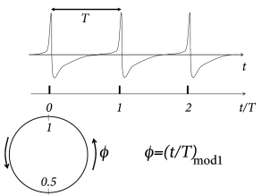
Suppose a neuron driven by a constant input fires regularly with period $T$ , i.e., it evolves on a periodic limit cycle. We have already seen in Ch. 4 that the position on the limit cycle can be represented by a phase $\phi$ . In contrast to Ch. 4 , we adopt here the conventions that (i) spikes occur at phase $\phi=0$ (Fig. 20.8 ) and (ii) between spikes the phase increases from zero to one at a constant speed $f_{0}=1$ , where $f_{0}=1/T$ is the frequency of the periodic firing. In more formal terms, the phase of an uncoupled neural ‘oscillator’ evolves according to the differential equation

{{\text{d}}\over{\text{d}}t}\phi=f_{0}\,

(20.13)

and we identify the value 1 with zero. Integration yields $\phi(t)=(t/T)_{{\rm mod}_{1}}$ where ‘mod ${}_{1}$ ’ means ‘modulo 1’. The phase $\phi$ represents the position on the limit cycle (Fig. 20.8 A).

Phase models for networks of $N$ interacting neurons are characterized by the intrinsic frequencies $f_{j}$ of the neurons ( $1\leq j\leq N$ ) as well as the mutual coupling. For weak coupling, the interaction can be directly formulated for the phase variables $\phi_{j}$

{{\text{d}}\over{\text{d}}t}\phi_{i}=f_{i}+\epsilon\sum_{j}w_{ij}P(\phi_{i},% \phi_{j})

(20.14)

where $\epsilon\ll 1$ is the overall coupling strength, $w_{ij}$ are the relative pairwise coupling, and $P$ the phase coupling function. For pulse-coupled oscillators, an interaction from neuron $j$ to neuron $i$ happens only at the moment when the presynaptic neuron $j$ emits a spike. Hence the phase coupling function $P(\phi_{i},\phi_{j})$ is replaced by

P(\phi_{i},\phi_{j})\longrightarrow F(\phi_{i})\sum_{f}\delta(t-t_{j}^{(f)})\,,

(20.15)

where $\{t_{j}^{(1)},t_{j}^{(2)},t_{j}^{(3)},\dots\}$ are the spike times of the presynaptic neuron, defined by the zero-crossings of $\phi_{j}$ , i.e., $\{t\,|\,\phi_{j}(t)=0\}$ . The function $F$ is the ‘phase response curve’: the effect of an input pulse depends on the momentary state (i.e. the phase $\phi_{i}$ ) of the receiving neuron (see the following example).

For neurons with synaptic currents of finite duration, phase coupling is not restricted to the moment of spike firing ( $\phi_{j}=0$ ) of the presynaptic neuron, but extends also to phase values $\phi_{j}>0$ . The phase coupling can be positive or negative. Positive values of $P$ lead to a phase advance of the postsynaptic neuron. Phase models are widely used to study synchronization phenomena ( 397 ) .

Example: Phase response curve

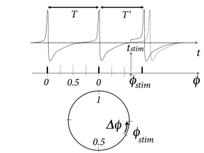
The idea of a phase response curve is illustrated in Fig. 20.8 B. A short positive stimulating input pulse of amplitude $\epsilon$ perturbs the period of an oscillator from its reference value $T$ to a new value $T^{\prime}$ which might be shorter or longer than $T$ ( 87; 555 ) . The phase response curve $\tilde{F}(\phi_{\rm stim})$ measures the phase advance $\Delta\phi=(T-T^{\prime})/T$ as a function of the phase $\phi_{\rm stim}$ at which the stimulus was given.

Knowledge of the stimulation phase is, however, not sufficient to characterize the effect on the period, because a stimulus of amplitude $2\epsilon$ is expected to cause a larger phase shift than a stimulus of amplitude $1\epsilon$ . The mathematically relevant notion is therefore the phase advance, divided by the (small) amplitude $\epsilon$ of the stimulus. More precisely, the infinitesimal phase response curve is defined as

F(\phi_{\rm stim})=\lim_{\epsilon\to 0}{T-T^{\prime}(\phi_{\rm stim})\over% \epsilon\,T}\,.

(20.16)

The infinitesimal phase response curve can be extracted from experimental data ( 201 ) and plays an important role in the theory of weakly coupled oscillators.

Example: Kuramoto model

The Kuramoto model ( 282; 8 ) describes a network of $N$ phase oscillators with homogeneous all-to-all connections $w_{ij}=J_{0}/N$ and a sinusoidal phase coupling function

{{\text{d}}\over{\text{d}}t}\phi_{i}=f_{i}+{J_{0}\over N}\sum_{j=1}^{N}\sin(2% \pi(\phi_{j}-\phi_{i}))

(20.17)

where $f_{i}$ is the intrinsic frequency of oscillator $i$ . For the analysis of the system, it is usually assumed that both the coupling strength $J_{0}$ and the frequency spread $(f_{i}-\overline{f})/\overline{f}$ are small. Here $\overline{f}$ denotes the mean frequency.

If the spread of intrinsic frequencies is zero, then an arbitrary small coupling $J_{0}>0$ synchronizes all units at the same phase $\phi_{i}(t)=\phi(t)=\overline{f}\,t$ . This is easy to see. First, synchronous dynamics $\phi_{i}(t)=\phi_{j}(t)=\phi(t)$ for all $i,j$ are a solution of Eq. ( 20.17 ). Second, if one of the oscillators is late by a small amount, say oscillator $n$ has a phase $\phi_{n}(t)<\phi(t)$ , then the interaction with the others makes it speed up (if the phase difference is smaller than $0.5$ ) or slow down (if the phase difference is larger than $0.5$ , until it is synchronized with the group of other neurons. More generally, for a fixed (small) spread of intrinsic frequencies, there is a minimal coupling strength $J_{c}$ above which global synchronization sets in.

We note that, in contrast to pulse-coupled models, units in the Kuramoto model can interact at arbitrary phases.

20.2.4 Synaptic plasticity and oscillations

Fig. 20.9: Network oscillations and STDP. A Top. During a near-synchronous oscillations, presynaptic spike timings $t^{f}$ have a jitter $\sigma$ with respect to the spike of a given postsynaptic neuron. Bottom: Because of axonal transmission delay, the spike arrival time $t^{\rm pre}=t^{f}+\Delta^{\rm ax}$ of presynaptic spikes at the synapse, is slightly shifted (light shaded area) to the regime ’post-before-pre’. Therefore, for an antisymmetric STDP window, synaptic depression dominates; compare the dark shaded areas for potentiation and depression. B. Same as in A, except that the amplitude of potentiation for near-synchronous firing is larger. As before, the total area under the STDP curve is balanced between potentiation and depression (integral over the STDP curve vanishes). C. Same as in B, except that the integral over the STDP curve is now positive, as is likely to be the case at high firing rates. For large jitter $\sigma$ potentiation dominates over depression (compare the dark-shaded areas).

During an oscillation a large fraction of excitatory neurons fires near-synchronously (Fig. 20.4 ). What happens to the oscillation if the synaptic efficacies between excitatory neurons are not fixed but subject to spike-timing dependent plasticity (STDP)? In this subsection we sketch some of the theoretical arguments ( 309; 395 )

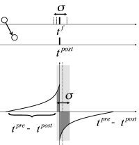
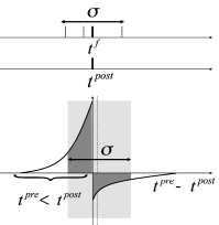
In Fig. 20.9 near synchronous spikes in a pair of pre- and postsynaptic neurons are shown together with a schematic STDP window; cf. Sect. 19.1.2 in Ch. 19 . Note that the horizontal axis of the STDP window is the difference between the spike arrival time $t^{\rm pre}$ at the presynaptic terminal and the spike firing time $t_{i}^{(f)}=t^{\rm post}$ of the postsynaptic neuron. This choice (where the presynaptic spike arrival time is identified with the onset of the EPSP) corresponds to one option, but other choices ( 328; 483 ) are equally common. With our convention, the jump from potentiation to depression occurs if postsynaptic firing coincides with presynaptic spike arrival. However, because of axonal transmission delays synchronous firing leads to spike arrival that is delayed with respect to the postsynaptic spike. Therefore, consistent with experiments ( 483 ) , synchronous spike firing with small jitter leads, at low repetition frequency, to a depression of synapses (Fig. 20.9 A). Lateral connections within the population of excitatory neurons are therefore weakened ( 309 ) .

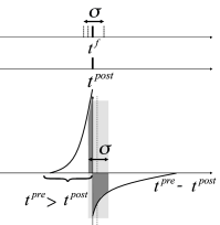
However, the shape of the STDP window is frequency dependent with a marked dominance of potentiation at high repetition frequencies ( 483 ) . Therefore, near-synchronous firing with a large jitter $\sigma$ leads to a strengthening of excitatory connections (Fig. 20.9 C) in the synchronously firing group ( 395 ) . In summary, synchronous firing and STDP tightly interact.

Example: Bistability of plastic networks

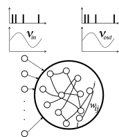
Since we are interested in the interaction of STDP with oscillations, we focus on a recurrent network driven by periodically modulated spike input (Fig. 20.10 A). The lateral connection weights $w_{ij}$ from a presynaptic neuron $j$ to a postsynaptic neuron $i$ are changed according to Eq. ( 19.2.2 ) of Chapter 19 , which we repeat here for convenience

	$\displaystyle\frac{{\text{d}}}{{\text{d}}t}w_{ij}(t)=$	$\displaystyle S_{j}(t)\,\left[a_{1}^{\text{pre}}+\int_{0}^{\infty}A_{-}(w_{ij}% )W_{-}(s)\,S_{i}(t-s)\;{\text{d}}s\right]$
		$\displaystyle+S_{i}(t)\,\left[a_{1}^{\text{post}}+\int_{0}^{\infty}A_{+}(w_{ij% })W_{+}(s)\,S_{j}(t-s)\;{\text{d}}s\right]\,,$		(20.18)

where $S_{j}=\sum_{f}\delta(t-t_{j}^{(f)})$ and $S_{i}=\sum_{f}\delta(t-t_{i}^{(f)})$ denote the spike trains of pre- and postsynaptic neurons, respectively. The time course of the STDP window is given by $W_{\pm}=\exp(-s/\tau_{\pm})$ and $a_{1}^{\text{pre}}$ and $a_{1}^{\text{post}}$ are non-Hebbian contributions, i.e., an isolated presynaptic or postsynaptic spike causes a small weight change, even if it is not paired with activity of the partner neuron. Non-Hebbian terms $a_{1}^{\text{pre}}+a_{1}^{\text{post}}<0$ are linked to ‘homeostatic’ or ‘heterosynaptic’ plasticity and are useful to balance weight growth caused by Hebbian terms (Ch. 19 ). The amplitude factors $A_{\pm}$ are given by soft-bounds analogous to Eq. 19.4 :

	$\displaystyle A_{+}(w_{ij})$	$\displaystyle=$	$\displaystyle A_{+}^{0}\,(w^{\rm max}-w_{ij})^{\beta}\,\quad{\rm for~{}}0<w<w^% {\rm max}$		(20.19)
	$\displaystyle A_{-}(w_{ij})$	$\displaystyle=$	$\displaystyle A_{-}^{0}\,(w_{ij})^{\beta}\,\qquad\qquad{\rm for~{}}0<w<w^{\rm max}$		(20.20)

with $\beta=0.05$ . An exponent $\beta$ close to zero implies that there is hardly any weight dependence except close to the bounds at zero and $w^{\rm max}$ .

The analysis of the network dynamics in the presence of STDP ( 395; 187; 256 ) shows that the most relevant quantities are (i) the integral over the STDP window $A_{+}(w)\tau_{+}+A_{-}(w)\tau_{-}$ evaluated at a value $w$ far away from the bounds; (ii) the Fourier transform of the STDP window at the frequency $1/T$ where $T$ is the period of the oscillatory drive; (iii) the sum of the non-Hebbian terms $a_{1}^{\text{pre}}+a_{1}^{\text{post}}$ .

Oscillations of brain activity in the $\delta$ or $\theta$ frequency band are relatively slow compared to the time scale of STDP. If we restrict the analysis to oscillations with a period $T$ that is long compared to the time scale $\tau_{+/-}$ of the learning window, the Fourier transform of the STDP window mentioned in (ii) can be approximated by the integral mentioned in (i). Note that slow sinusoidal oscillations correspond to a large jitter $\sigma$ of spike times (Fig. 20.9 C).

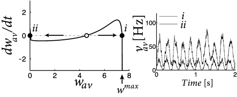
Pfister and Tass ( 395 ) found that the network dynamics is bistable if the integral over the learning window is positive (which causes an increase of weights for uncorrelated Poisson firing), but weight increase is counterbalanced by weight decrease caused by homeostatic terms in the range $C<a_{1}^{\text{pre}}+a_{1}^{\text{post}}<c<0$ with suitable negative constants $C$ and $c$ . Therefore, for the same periodic stimulation stimulation paradigm, the network can be in either a stable state where the average weight is close to zero, or in a different stable state where the average weight is significantly positive (Fig. 20.10 B). In the latter case, the oscillation amplitude in the network is enhanced (Fig. 20.10 C).