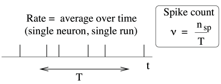
The first and most commonly used definition of a firing rate refers to a temporal average. An experimentalist observes in trial $k$ the spikes of a given neuron (see Fig. 7.6). The firing rate in trial $k$ is the spike count $n_{k}^{\rm sp}$ in an interval of duration $T$ divided by $T$.

The length $T$ of the time window is set by the experimenter and depends on the type of neuron and the stimulus. In practice, to get sensible averages, several spikes should occur within the time window. Typical values are $T=100$ ms or $T=500$ ms, but the duration may also be longer or shorter.

This definition of rate has been successfully used in many preparations, particularly in experiments on sensory or motor systems. A classical example is the stretch receptor in a muscle spindle (9). The number of spikes emitted by the receptor neuron increases with the force applied to the muscle.

If the same experiment is repeated several times, the measured spike count varies between one trial and the next. Let us denote the spike count in trial $k$ by the variable $n^{\rm sp}_{k}$, its mean by $\langle n^{\rm sp}\rangle$ and deviations from the mean as $\Delta n^{\rm sp}_{k}=n^{\rm sp}_{k}-\langle n^{\rm sp}\rangle$. Variability of the spike count measure is characterized by the Fano Factor, defined as the variance of the spike count $\langle(\Delta n^{\rm sp})^{2}\rangle$ divided by its mean

In experiments, the mean and variance are estimated by averaging over $K$ trials $\langle n^{\rm sp}\rangle=(1/K)\sum_{k=1}^{K}\,n^{\rm sp}_{k}$ and $\langle(\Delta n^{\rm sp})^{2}\rangle=(1/K)\sum_{k=1}^{K}\,(\Delta n^{\rm sp}_{k})^{2}$.

If we find on average $\langle n^{\rm sp}\rangle$ spikes in a long temporal window of duration $T$, the mean interval between two subsequent spikes is $T/\langle n^{\rm sp}\rangle$. Indeed, using the notion of interspike-interval distribution to be introduced below (Section 7.3), we can make the following statement: the firing rate defined here as spike count divided by the measurement time $T$ is identical to the inverse of the mean interspike interval. We will come back to interspike intervals in Section 7.3.

It is tempting, but misleading, to consider the inverse interspike interval as a ’momentary firing rate’: if a first spike occurs at time $t^{(k)}$ and the next one at time $t^{(k+1)}$, we could artificially assign a variable $\tilde{\nu}(t)=1/(t^{(k+1)}-t^{(k)})$ for all times $t^{(k)}<t\leq t^{(k)}$. However, the temporal average of $\tilde{\nu}(t)$ over a much longer time $T$ is not the same as a the mean rate $\nu$ defined here as spike count divided by $T$, simply because $1/\langle x\rangle\neq\langle(1/x)\rangle$. A practical definition of ’instantaneous firing rate’ will be given below in Section 7.2.2.

An experimenter records from a neuron while stimulating with some input sequence. The same stimulation sequence is repeated several times and the neuronal response is reported in a Peri-Stimulus-Time Histogram (PSTH) with bin width $\Delta t$; see Fig. 7.7. The time $t$ is measured with respect to the start of the stimulation sequence and $\Delta t$ defines the time bin for generating the histogram, it is typically on the order of milliseconds.

The number of occurrences of spikes $n_{K}(t;t+\Delta t)$ summed over all repetitions of the experiment divided by the number $K$ of repetitions is a measure of the typical activity of the neuron between time $t$ and $t+\Delta t$. A further division by the interval length $\Delta t$ yields the spike density

Sometimes the result is smoothed to get a continuous (time-dependent) rate variable, usually reported in units of Hz. As an experimental procedure, the PSTH measure is a useful method to evaluate neuronal activity, in particular in the case of time-dependent stimuli; see Fig. 7.4. We call it the time-dependent firing rate.

In order to see the relation of Eq. 7.6 to a time-dependent firing rate, we recall that spikes are formal events characterized by their firing time $t^{(f)}$ where $f$ counts the spikes. In Chapter 1 we have defined (Eq. (1.14)) the spike train as a sum of $\delta$-functions:

If each stimulation can be considered as an independent sample from the identical stochastic process, we can define an instantaneous firing rate as an expectation over trials

An expectation value over $\delta$-functions may look weird to the reader not used to seeing such mathematical objects. Let us therefore consider the experimental procedure to estimate the expectation value. First, in each trial $k$, we count the number of spikes that occur in a short time interval $\Delta t$ by integrating the spike train over time, $n^{\rm sp}_{k}(t)=\int_{t}^{t+\Delta t}S_{k}(t^{\prime}){\text{d}}t^{\prime}$ where the lower index $k$ denotes the trial number. Note that integration removes the $\delta$-function. Obviously, if the time bin $\Delta t$ is small enough we will find at most one spike so that $n^{\rm sp}_{k}$ is either zero or one. Second, we average over the $K$ trials and divide by $\Delta t$ in order to have the empirical estimate

The PSTH, defined as spike count per time bin averaged over several trials and divided by the bin length (the right-hand side of Eq. (7.9)), provides therefore an empirical estimate of the instantaneous firing rate (the left-hand side).

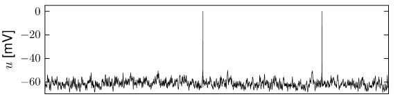
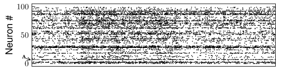
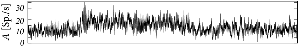
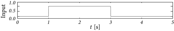
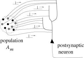
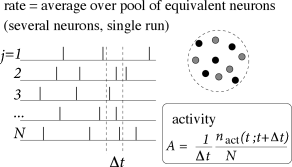
The number of neurons in the brain is huge. Often many neurons have similar properties and respond to the same stimuli. For example, neurons in the primary visual cortex of cats and monkeys are arranged in columns of cells with similar properties (230). Let us idealize the situation and consider a population of neurons with identical properties. In particular, all neurons in the population should have the same pattern of input and output connections. The spikes of the neurons in a population $m$ are sent off to another population $n$. In our idealized picture, each neuron in population $n$ receives input from all neurons in population $m$. The relevant quantity, from the point of view of the receiving neuron, is the proportion of active neurons in the presynaptic population $m$; see Fig. 7.8A. Formally, we define the population activity

where $N$ is the size of the population, $n_{\rm act}(t;t+\Delta t)$ is the number of spikes (summed over all neurons in the population) that occur between $t$ and $t+\Delta t$ where $\Delta t$ is a small time interval; see Fig. 7.8. Eq. (7.11) defines a variable with units inverse time – in other words, a rate.

As we can see from Fig. 7.5C, the population activity may vary rapidly and can reflect changes in the stimulus conditions nearly instantaneously. Before we discuss the problem of neural coding (Section 7.6), let us first study further statistical measures of spike train statistics.