8 Noisy Input Models: Barrage of Spike Arrivals 8.2 Stochastic spike arrival 8.4 Diffusion limit and Fokker-Planck equation(*)

8.3 Subthreshold vs. Superthreshold regime

One of the aims of noisy neuron models is to mimic the large variability of interspike intervals found, e.g., in vertebrate cortex. To arrive at broad interval distributions, it is not just sufficient to introduce noise into a neuron model. Apart from the noise level, other neuronal parameters such as the firing threshold or a bias current have to be tuned so as to make the neuron sensitive to noise. In this section we introduce a distinction between super- and subthreshold stimulation (7; 470; 283; 520; 82).

An arbitrary time-dependent stimulus $I(t)$ is called subthreshold, if it generates a membrane potential that stays – in the absence of noise – below the firing threshold. Due to noise, however, even subthreshold stimuli can induce action potentials. Stimuli that induce spikes even in a noise-free neuron are called superthreshold.

The distinction between sub- and superthreshold stimuli has important consequences for the firing behavior of neurons in the presence of noise. To see why, let us consider a leaky integrate-and-fire neuron with constant input $I_{0}$ for $t>0$ . Starting from $u(t=0)=u_{r}$ , the trajectory of the membrane potential is

u_{0}(t)=u_{\infty}\,\left[1-e^{-t/\tau_{m}}\right]+u_{r}\,e^{-t/\tau_{m}}\,.

(8.33)

In the absence of a threshold, the membrane potential approaches the value $u_{\infty}=R\,I_{0}$ for $t\to\infty$ . If we take the threshold $\vartheta$ into account, two cases may be distinguished. First, if $u_{\infty}<\vartheta$ (subthreshold stimulation), the neuron does not fire at all. Second, if $u_{\infty}>\vartheta$ (superthreshold stimulation), the neuron fires regularly. The interspike interval is $s_{0}$ derived from $u_{0}(s_{0})=\vartheta$ . Thus

s_{0}=\tau\,{\rm ln}{u_{\infty}-u_{r}\over u_{\infty}-\vartheta}\,.

(8.34)

We now add diffusive noise. In the superthreshold regime, noise has little influence, except that it broadens the interspike interval distribution. Thus, in the superthreshold regime, the spike train in the presence of diffusive noise, is simply a noisy version of the regular spike train of the noise-free neuron.

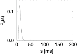
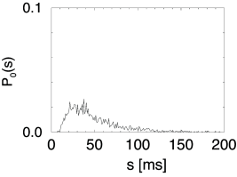
On the other hand, in the subthreshold regime, the spike train changes qualitatively, if noise is switched on; see (283) for a review. Stochastic background input turns the quiescent neuron into a spiking one. In the subthreshold regime, spikes are generated by the fluctuations of the membrane potential, rather than by its mean (7; 470; 520; 82; 148). The interspike interval distribution is therefore broad; see Fig. 8.7.

Fig. 8.7: Integrate-and-fire neuron ( $\tau_{m}=10\,$ ms) with superthreshold (left column) and subthreshold (right column) stimulation. A. Without noise, a neuron with superthreshold stimulus $I_{a}$ fires regularly. Spikes are marked by vertical lines. The threshold is indicated by a horizontal line. The dashed line shows the evolution of the membrane potential in the absence of the threshold. B. The same neuron with subthreshold stimulation $I_{b}$ does not fire. C. If we add stochastic excitatory and inhibitory spike input ( $w_{\pm}=0.05$ at $\nu_{\pm}=1.6~{}$ kHz) to the constant input $I_{a}$ , the membrane potential drifts away from the noise-free reference trajectory, but firing remains fairly regular. D. The same sequence of input spikes added to the subthreshold current $I_{b}$ generates irregular spiking. E and F. Histogram of interspike intervals in C and D, respectively, as an estimator of the interval distribution $P_{0}(s)$ in the super- and subthreshold regime. The mean interval $\langle s\rangle$ is 12 ms (E) and 50 ms (F); the $C_{V}$ values are 0.30 and 0.63, respectively.

Example: Interval distribution in the superthreshold regime

For small noise amplitude $0<\sigma\ll u_{\infty}-\vartheta$ , and superthreshold stimulation, the interval distribution is centered at the deterministic interspike interval $s_{0}$ . Its width can be estimated from the width of the fluctuations ${\langle\Delta u^{2}_{\infty}\rangle}$ of the free membrane potential; cf. Eq. (8.13). After the reset, the variance of the distribution of membrane potentials is zero and increases slowly thereafter. As long as the mean trajectory is far away from the threshold, the distribution of membrane potentials has a Gaussian shape.

As time goes on, the distribution of membrane potentials is pushed across the threshold. Since the membrane potential crosses the threshold with slope $u_{0}^{\prime}$ , there is a scaling factor $u_{0}^{\prime}={\text{d}}u_{0}(t)/{\text{d}}t$ evaluated at $t=s_{0}$ between the (approximately) Gaussian distribution of membrane potential and the interval distribution; cf. Fig. 8.8. The interval distribution is therefore also approximately given by a Gaussian with mean $s_{0}$ and width $\sigma/\sqrt{2}\,u_{0}^{\prime}$ (525), i.e.,

P_{0}(t|0)={1\over\sqrt{\pi}}{u_{0}^{\prime}\over\sigma}\exp\left[-{(u_{0}^{% \prime})^{2}\,(t-s_{0})^{2}\over\sigma^{2}}\right]\,.

(8.35)