1.3 Integrate-And-Fire Models
We have seen in the previous section that, to a first and rough approximation, neuronal dynamics can be conceived as a summation process (sometimes also called ‘integration’ process) combined with a mechanism that triggers action potentials above some critical voltage. Indeed in experiments firing times are often defined as the moment when the membrane potential reaches some threshold value from below. In order to build a phenomenological model of neuronal dynamics, we describe the critical voltage for spike initiation by a formal threshold . If the voltage (that contains the summed effect of all inputs) reaches from below, we say that neuron fires a spike. The moment of threshold crossing defines the firing time .
The model makes use of the fact that neuronal action potentials of a given neuron always have roughly the same form. If the shape of an action potential is always the same, then the shape cannot be used to transmit information: rather information is contained in the presence or absence of a spike. Therefore action potentials are reduced to ‘events’ that happen at a precise moment in time.
Neuron models where action potentials are described as events are called ’Integrate-and-Fire’ models. No attempt is made to describe the shape of an action potential. Integrate-and-fire models have two separate components that are both necessary to define their dynamics: first, an equation that describes the evolution of the membrane potential ; and second, a mechanism to generate spikes.
In the following we introduce the simplest model in the class of integrate-and-fire models using the following two ingredients: (i) a linear differential equation to describe the evolution of the membrane potential; (ii) a threshold for spike firing. This model is called the ‘Leaky Integrate-and-Fire’ Model. Generalized integrate-and-fire models that will be discussed in Part II of the book can be seen as variations of this basic model.
1.3.1 Integration of Inputs
The variable describes the momentary value of the membrane potential of neuron . In the absence of any input, the potential is at its resting value . If an experimentalist injects a current into the neuron, or if the neuron receives synaptic input from other neurons, the potential will be deflected from its resting value.
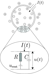
In order to arrive at an equation that links the momentary voltage to the input current , we use elementary laws from the theory of electricity. A neuron is surrounded by a cell membrane, which is a rather good insulator. If a short current pulse is injected into the neuron, the additional electrical charge has to go somewhere: it will charge the cell membrane (Fig. 1.6A). The cell membrane therefore acts like a capacitor of capacity . Because the insulator is not perfect, the charge will, over time, slowly leak through the cell membrane. The cell membrane can therefore be characterized by a finite leak resistance .
The basic electrical circuit representing a leaky integrate-and-fire model consists of a capacitor in parallel with a resistor driven by a current ; see Fig. 1.6.
| A | B | ||
|---|---|---|---|
|
 |
If the driving current vanishes, the voltage across the capacitor is given by the battery voltage . For a biological explanation of the battery we refer the reader to the next chapter. Here we have simply inserted the battery ‘by hand’ into the circuit so as to account for the resting potential of the cell (Fig. 1.6A).
In order to analyze the circuit, we use the law of current conservation and split the driving current into two components,
| (1.3) |
The first component is the resistive current which passes through the linear resistor . It can be calculated from Ohm’s law as where is the voltage across the resistor. The second component charges the capacitor . From the definition of the capacity as (where is the charge and the voltage), we find a capacitive current . Thus
| (1.4) |
We multiply Eq. (1.4) by and introduce the time constant of the ‘leaky integrator’. This yields the standard form
| (1.5) |
We refer to as the membrane potential and to as the membrane time constant of the neuron.
From the mathematical point of view, Eq. (1.5) is a linear differential equation. From the point of view of an electrical engineer, it is the equation of a leaky integrator or -circuit where resistor and capacitor are arranged in parallel. From the point of view of the neuroscientist, Eq. (1.5) is called the equation of a passive membrane.
What is the solution of Eq. (1.5)? We suppose that, for whatever reason, at time the membrane potential takes a value . For the input vanishes . Intuitively we expect that, if we wait long enough, the membrane potential relaxes to its resting value . Indeed, the solution of the differential equation with initial condition is
| (1.6) |
Thus, in the absence of input, the membrane potential decays exponentially to its resting value. The membrane time constant is the characteristic time of the decay. For a typical neuron it is in the range of 10ms, and hence rather long compared to the duration of a spike which is on the order of 1ms.
The validity of the solution (1.6) can be checked by taking the derivative on both sides of the equation. Since it is the solution in the absence of input, it is sometimes called the ‘free’ solution.
1.3.2 Pulse Input
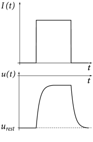
Before we continue with the definition of the integrate-and-fire model and its variants, let us study the dynamics of the passive membrane defined by Eq. (1.5) in a simple example. Suppose that the passive membrane is stimulated by a constant input current which starts at and ends at time . For the sake of simplicity we assume that the membrane potential at time is at its resting value .
As a first step, let us calculate the time course of the membrane potential. The trajectory of the membrane potential can be found by integrating (1.5) with the initial condition . The solution for is
| (1.7) |
If the input current never stopped, the membrane potential (1.7) would approach for the asymptotic value . We can understand this result by looking at the electrical diagram of the -circuit in Fig. 1.6. Once a steady state is reached, the charge on the capacitor no longer changes. All input current must then flow through the resistor. The steady-state voltage at the resistor is therefore so that the total membrane voltage is .
Example: Short pulses and the Dirac function
For short pulses the steady state value is never reached. At the end of the pulse, the value of the membrane potential is given according to Eq. (1.7) by For pulse durations (where means much smaller than) we can expand the exponential term into a Taylor series: . To first order in we find
| (1.8) |
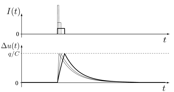
Thus, the voltage deflection depends linearly on the amplitude and the duration of the pulse (Fig. 1.7).
We now make the duration of the pulse shorter and shorter while increasing the amplitude of the current pulse to a value , so that the integral remains constant. In other words, the total charge delivered by the current pulse is always the same. Interestingly, the voltage deflection at the end of the pulse calculated from Eq. (1.8) remains unaltered, however short we make the pulse. Indeed, from Eq. (1.8) we find where we have used . Thus we can consider the limit of an infinitely short pulse
| (1.9) |
is called the Dirac -function. It is defined by for and .
Obviously, the Dirac -function is a mathematical abstraction since it is practically impossible to inject a current with an infinitely short and infinitely strong current pulse into a neuron. Whenever we encounter a -function, we should remember that, as a stand-alone object, it looks strange, but becomes meaningful as soon as we integrate over it. Indeed the input current defined in Eq. (1.9) needs to be inserted into the differential equation (1.5) and integrated. The mathematical abstraction of the Dirac function suddenly makes a lot of sense, because the voltage change induced by a short current pulse is always the same, whenever the duration of the pulse is much shorter than the time constant . Thus, the exact duration of the pulse is irrelevant, as long as it is short enough.
With the help of the -function, we no longer have to worry about the time course of the membrane potential during the application of the current pulse: the membrane potential simply jumps at time by an amount . Thus, it is as if we added instantaneously a charge onto the capacitor of the circuit.
What happens for times ? The membrane potential evolves from its new initial value in the absence of any further input. Thus we can use the ‘free’ solution from Eq. (1.6) with and .
We can summarize the considerations of this subsection by the following statement. The solution of the linear differential equation with pulse input
| (1.10) |
is for and given by
| (1.11) |
The right-hand side of the equation is called the impulse-response function or Green’s function of the linear differential equation.
1.3.3 The Threshold for Spike Firing
Throughout this book, the term ‘firing time’ refers to the moment when a given neuron emits an action potential . The firing time in the leaky integrate-and-fire model is defined by a threshold criterion
| (1.12) |
The form of the spike is not described explicitly. Rather, the firing time is noted and immediately after the potential is reset to a new value ,
| (1.13) |
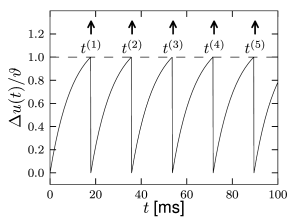
For the dynamics is again given by (1.5) until the next threshold crossing occurs. The combination of leaky integration (1.5) and reset (1.13) defines the leaky integrate-and-fire model (495). The voltage trajectory of a leaky integrate-and-fire model driven by a constant current is shown in Fig. 1.9.
For the firing times of neuron we write where is the label of the spike. Formally, we may denote the spike train of a neuron as the sequence of firing times
| (1.14) |
where is the Dirac function introduced before, with for and . Spikes are thus reduced to points in time (Fig. 1.8). We remind the reader that the -function is a mathematical object that needs to be inserted into an integral in order to give meaningful results.
| A | B |
|---|---|
|
 |
1.3.4 Time-dependent Input (*)22Sections marked by an asterisk are mathematically more advanced and can be omitted during a first reading of the book.
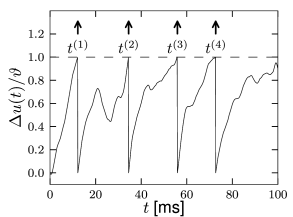
We study a leaky integrate-and-fire model which is driven by an arbitrary time-dependent input current ; cf. Fig. 1.9B. The firing threshold has a value and after firing the potential is reset to a value .
In the absence of a threshold, the linear differential equation (1.5) has a solution
| (1.15) |
where is an arbitrary input current and is the membrane time constant. We assume here that the input current is defined for a long time back into the past: so that we do not have to worry about the initial condition. A sinusoidal current or a step current pulse, where denotes the Heaviside step function with for and for , are two examples of a time-dependent current, but the solution, Eq. (1.15), is also valid for every other time-dependent input current.
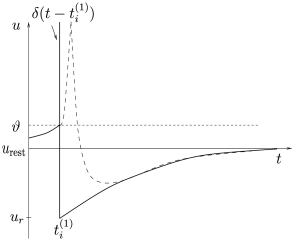
So far our leaky integrator does not have a threshold. What happens to the solution Eq. (1.15), if we add a threshold ? Each time the membrane potential hits the threshold, the variable is reset from to . In the electrical circuit diagram, the reset of the potential corresponds to removing a charge from the capacitor (Fig. 1.6) or, equivalently, adding a negative charge onto the capacitor. Therefore, the reset corresponds to a short current pulse at the moment of the firing . Indeed, it is not unusual to say that a neuron ‘discharges’ instead of ‘fires’. Since the reset happens each time the neuron fires, the reset current is
| (1.16) |
where denotes the spike train, defined in Eq. (1.14).
The short current pulse corresponding to the ‘discharging’ is treated mathematically just like any other time-dependent input current. The total current , consisting of the stimulating current and the reset current, is inserted into the solution (1.15) to give the final results
| (1.17) |
where the firing times are defined by the threshold condition
| (1.18) |
Note that with our definition of the Dirac -function in Eq. (1.9), the discharging reset follows immediately after the threshold crossing, so that the natural sequence of events – first firing, then reset – is respected.
Eq. (1.17) looks rather complicated. It has, however, a simple explanation. In Sect. 1.3.2 we have seen that a short input pulse at time causes at time a response of the membrane proportional to , sometimes called the impulse response function or Green’s function; cf. Eq. (1.11). The second term on the right-hand side of Eq. (1.17) is the effect of the discharging current pulses at the moment of the reset.
In order to interpret the last term on the right-hand side, we think of a stimulating current as consisting of a rapid sequence of discrete and short current pulses. In discrete time, there would be a different current pulse in each time step. Because of the linearity of the differential equation, the effect of all these short current pulses can be added. When we return from discrete time to continuous time, the sum of the impulse response functions turns into the integral on the right-hand side of Eq. (1.17).
1.3.5 Linear Differential Equation vs. Linear Filter: Two Equivalent Pictures (*)
The leaky integrate-and-fire model is defined by the differential equation (1.5), i.e.,
| (1.19) |
combined with the reset condition
| (1.20) |
where are the firing times
| (1.21) |
As we have seen in the previous subsection, the linear equation can be integrated and yields the solution (1.17). It is convenient to rewrite the solution in the form
| (1.22) |
where we have introduced filters and . Interestingly, Eq. (1.22) is much more general than the leaky integrate-and-fire model, because the filters do not need to be exponentials but could have any arbitrary shape. The filter describes the reset of the membrane potential and, more generally, accounts for neuronal refractoriness. The filter summarizes the linear electrical properties of the membrane. Eq. (1.22) in combination with the threshold condition (1.21) is the basis of the Spike Response Model and Generalized Linear Models, which will be discussed in Part II.
1.3.6 Periodic drive and Fourier transform (*)
Formally, the complex Fourier transform of a real-valued function with argument on the real line is
| (1.23) |
where and are called amplitude and phase of the Fourier transform at frequency . The mathematical condition for a well-defined Fourier transform is that the function be Lebesgue integrable with integral . If is a function of time, then is a function of frequency. An inverse Fourier transform leads back from frequency-space to the original space, i.e., time.
For a linear system, the above definition gives rise to several convenient rules for Fourier-transformed equations. For example, let us consider the system
| (1.24) |
where is a real-valued input (e.g., a current), the real-valued system output (e.g., a voltage) and a linear response filter, or kernel, with for because of causality. The convolution on the right-hand side of Eq. (1.24) turns after Fourier transformation into a simple multiplication, as shown by the following steps of calculation:
| (1.25) | |||||
where we introduced in the last step the variable and used the definition (1.23) of the Fourier transform.
Similarly, the derivative of a function can be Fourier-transformed using the product rule of integration. The Fourier transform of the derivative of is .
While introduced here as a purely mathematical operation, it is often convenient to visualize the Fourier transform in the context of a physical system driven by a periodic input. Consider the linear system of Eq. (1.24) with an input
| (1.26) |
A short comment on the notation. If the input is a current, it should be real-valued, as opposed to a complex number. We therefore take as a real and positive number and focus on the real part of the complex equation (1.26) as our physical input. When we perform a calculation with complex numbers, we therefore implicitly assume that, at the very end, we only take the real part of solution. However, the calculation with complex numbers turns out to be convenient for the steps in between.
Inserting the periodic drive, Eq. (1.26), into Eq. (1.24) yields
| (1.27) |
Hence, if the input is periodic at frequency the output is so, too. The term in square brackets is the Fourier transform of the linear filter. We write . The ratio between the amplitude of the output and that of the input is
| (1.28) |
The phase of the Fourier-transformed linear filter corresponds to phase shift between input and output or, to say it differently, a delay where is the period of the oscillation. Fourier transforms will play a role in the discussion of signal processing properties of connected networks of neurons in Part III of the book.
Example: Periodic drive of a passive membrane
We consider the differential equation of the passive membrane defined in Eq. (1.5) and choose voltage units such that , i.e.,
| (1.29) |
The solution, given by Eq. (1.15), corresponds to the convolution of the input with a causal linear filter for . In order to determine the response amplitude to a periodic drive we need to calculate the Fourier transform of :
| (1.30) |
For the right-hand side is proportional to . Therefore the amplitude of the response to a periodic input decreases at high frequencies.