13 Continuity Equation and the Fokker-Planck Approach 13.1 Continuity equation 13.3 Fokker-Planck equation

13.2 Stochastic spike arrival

We consider the flux $J(u,t)$ in a homogeneous population of integrate-and-fire neurons with voltage equation (13.1). We assume that all neurons in the population receive the same driving current $I^{\rm ext}$ . In addition each neuron receives stochastic background input. We allow for different types of synapses. An input spike at a synapse of type $k$ causes a jump of the membrane potential by an amount $w_{k}$ . For example, $k=1$ could refer to weak excitatory synapses with jump size $w_{1}>0$ ; $k=2$ to strong excitatory synapses $w_{2}>w_{1}$ ; and $k=3$ to inhibitory synapses with $w_{3}<0$ . The effective spike arrival rate (summed over all synapses of the same type $k$ ) is denoted as $\nu_{k}$ . While the mean spike arrival rates $\nu_{k}(t)$ are identical for all neurons, we assume that the actual input spike trains at different neurons and different synapses are independent. In a simulation, spike arrival at different neurons could for example be simulated by independent Poisson processes with a common spike arrival rate $\nu(t)$ .

Whereas spike arrivals cause a jump of the membrane potential, a finite input current $I^{\rm ext}(t)$ generates a smooth drift of the membrane potential trajectories. In such a network, the flux $J(u,t)$ across a reference potential $u_{0}$ can therefore be generated in two different ways: through a ‘jump’ or a ‘drift’ of trajectories. We separate the two contributions to the flux into $J_{\rm jump}$ and $J_{\rm drift}$

J(u_{0},t)=J_{\rm drift}(u_{0},t)+J_{\rm jump}(u_{0},t)\,,

(13.9)

and treat each of these in turn.

Fig. 13.2: A. All trajectory that are less than $w_{k}$ below $u_{0}$ cross $u_{0}$ upon spike arrival. B. The drift $J_{\rm drift}(u_{0},t)$ depends on density of trajectories and on the slope with which the trajectories cross the boundary $u_{0}$ .

13.2.1 Jumps of membrane potential due to stochastic spike arrival

To evaluate $J_{\rm jump}$ , let us consider excitatory input $w_{k}>0$ . All neurons that have a membrane potential $u_{i}$ with $u_{0}-w_{k}<u_{i}\leq u_{0}$ will jump across the reference potential $u_{0}$ upon spike arrival at a synapse of type $k$ ; cf. Fig. 13.2A. Since at each neuron spikes arrive stochastically, we cannot predict with certainty whether a single neuron receives a spike around time $t$ or not. But because the rate $\nu_{k}$ of spike arrival at synapses of type $k$ is the same for each neuron, while the actual spike trains are independent for different neurons, the total (expected) flux, or probability current, caused by input spikes at all synapses can be calculated as

J_{\rm jump}(u_{0},t)=\sum_{k}\nu_{k}\,\int_{u_{0}-w_{k}}^{u_{0}}p(u,t)\,{% \text{d}}u\,.

(13.10)

If the number of neurons is large, the actual flux is very close to the expected flux given in Eq. 13.10.

13.2.2 Drift of membrane potential

The drift $J_{\rm drift}(u_{0},t)$ through the reference potential $u_{0}$ is given by the density $p(u_{0},t)$ at the potential $u_{0}$ times the momentary ‘velocity’ ${\text{d}}u/{\text{d}}t$ ; cf. Fig. 13.2B. Therefore

J_{\rm drift}(u_{0},t)=\left.{{\text{d}}u\over{\text{d}}t}\right|_{u_{0}}p(u_{% 0},t)={1\over\tau_{m}}\,[f(u_{0})+R\,I^{\rm ext}(t)]\,p(u_{0},t)\,,

(13.11)

where $f(u_{0})$ is the nonlinearity of the the integrate-and-fire model in Eq. (13.1). Note that synaptic $\delta$ -current pulses cause a jump of the membrane potential and therefore contribute only to $J_{\rm jump}$ (see Subsection 13.2.1), but not to the drift flux considered here. Current pulses of finite duration, however, should be included in $I^{\rm ext}(t)$ in Eq. (13.11).

Example: Leaky integrate-and-fire neurons

With $f(u)=-(u-u_{\rm rest})$ we have for leaky integrate-and-fire neurons a drift-induced flux

J_{\rm drift}(u_{0},t)={1\over\tau_{m}}\,[-u_{0}+u_{\rm rest}+R\,I^{\rm ext}(t% )]\,p(u_{0},t)\,.

(13.12)

13.2.3 Population activity

A positive flux through the threshold $\theta_{\rm reset}$ yields the population activity $A(t)$ . Since the flux has components from the drift and from the jumps, the total flux at the threshold is

A(t)={1\over\tau_{m}}\,[f(\theta_{\rm reset})+R\,I^{\rm ext}(t)]\,p(\theta_{% \rm reset},t)+\sum_{k}\nu_{k}\,\int_{\theta_{\rm reset}-w_{k}}^{\theta_{\rm reset% }}p(u,t)\,{\text{d}}u\,.

(13.13)

Since the probability density vanishes for $u>\theta_{\rm reset}$ , the sum over the synapses $k$ can be restricted to all excitatory synapses.

If we insert the explicit form of the flux that we derived in Eqs. (13.10) and (13.11) into the continuity equation (13.7), we arrive at the density equation for the membrane potential of integrate-and-fire neurons

$\displaystyle{\partial\over\partial t}p(u,t)$	$\displaystyle=$	$\displaystyle-{1\over\tau_{m}}\,{\partial\over\partial u}\left\{\left[f(u)+R\,% I^{\rm ext}(t)\right]\,p(u,t)\right\}$	(13.14)
		$\displaystyle+\sum_{k}\nu_{k}(t)\,\left[p(u-w_{k},t)-p(u,t)\right]$
		$\displaystyle+A(t)\,\delta(u-u_{r})-A(t)\,\delta(u-\theta_{\rm reset})\,.$

The first two terms on the right-hand side describe the continuous drift, the third term the jumps caused by stochastic spike arrival, and the last two terms take care of the reset. Because of the firing condition, we have $p(u,t)=0$ for $u>\theta_{\rm reset}$ .

Equations (13.13) and (13.14) can be used to predict the population activity $A(t)$ in a population of integrate-and-fire neurons stimulated by an arbitrary common input $I^{\rm ext}(t)$ . For a numerical implementation of Eq. (13.6) we refer the reader to the literature (367; 371).

Fig. 13.3: Solution of the membrane potential density equation for time dependent input. The input is sinusoidal with a period of 100ms. A. Population activity $A(t)$ (thick solid line; left vertical scale) in response to excitatory and inhibitory spikes arriving with modulated firing rates (thin solid and dashed lines, respectively; right vertical scale). B. The membrane population density $p(u,t)$ as a function of voltage and time during one period of the periodic stimulation; adapted from (367)

Example: Transient response of population activity

The population of 1 000 leaky integrate-and-fire neurons simulated by Nykamp and Tranchina (367) receives stochastic spike arrivals at excitatory and inhibitory synapses at rate $\nu_{E}(t)$ and $\nu_{I}(t)$ , respectively. Each input spike causes a voltage jump of amplitude $w$ . The raw jump size is drawn from some distribution and then multiplied with the difference between the synaptic reversal potential and value of the membrane potential just before spike arrival, so as to approximate the effect of conductance based synapses The average jump size in the simulation was about 0.5mV at excitatory synapses and -0.33mV at inhibitory synapses (367).

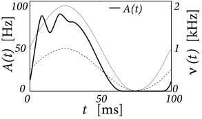
The input rates are periodically modulated with frequency $f=10$ Hz

\nu_{E/I}(t)=\bar{\nu}_{E/I}\,[1+\sin(2\pi\,f\,t)],

(13.15)

with $\bar{\nu}_{E}=2$ kHz and $\bar{\nu}_{I}=2$ kHz. Integration of the population equations (13.13) and (13.14) yields a population activity $A(t)$ that responds strongly during the rising phase of the input, well before the excitatory input reaches its maximum; cf. Fig. 13.3A.

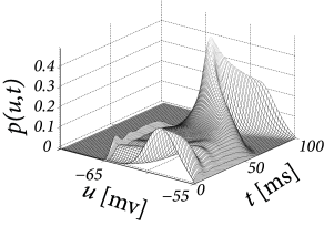
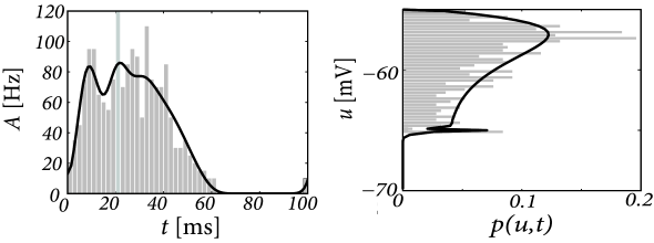
We compare the solution of the population activity equations with the explicit simulation of 1 000 uncoupled neurons. The simulated population activity of the finite network (Fig. 13.4A) is well approximated by the predicted activity $A(t)$ which becomes correct if the number of neurons goes to infinity. The density equations also predict the voltage distribution at each moment in time (Fig. 13.3B). The empirical histogram of voltages in a finite population of 1 000 neurons (Fig. 13.4B) is close to the smooth voltage distribution predicted by the theory.

Fig. 13.4: Comparison of theory and simulation. A. Population firing rate $A(t)$ as a function of time in a simulation of 1 000 neurons (histogram bars) compared to the prediction by the theory (solid line) while the population receives periodically modulated excitatory and inhibitory conductance input with period $T=100$ ms. B. Histogram of voltage distribution (gray horizontal bars) at $t_{0}=20$ ms in a population of 1 000 neurons compared to the solution $p(u,t_{0})$ of the density equation during the periodic stimulation; adapted from (367).

13.2.4 Single neuron versus population of neurons

Equation (13.14) that describes the dynamics of $p(u,t)$ in a population of integrate-and-fire neurons is nearly identical to that of a single integrate-and-fire neuron with stochastic spike arrival; cf. Eqs. (8.40) in Chapter 8. Apart from the fact that we have formulated the problem here for arbitrary nonlinear integrate-and-fire models, there are three subtle differences.

First, while $p(u,t)$ was introduced in Chapter 8 as probability density for the membrane potential of a single neuron, it is now interpreted as the density of membrane potentials in a large population of neurons.

Second, the normalization is different. In Chapter 8, we considered a single neuron which was initialized at time $\hat{t}$ at a voltage $u_{r}$ . For $t>t_{0}$ , the integrated density $\int_{-\infty}^{\theta_{\rm reset}}p(u,t)\,{\text{d}}u$ $\leq 1$ was interpreted as the probability that the neuron under consideration has not yet fired since its last spike at $\hat{t}$ . The value of the integral decreases therefore over time. In the present treatment of a population of neurons, a neuron remains part of the population even if it fires. Thus the integral over the density remains constant over time; cf. Eq. (13.3).

Third, the fraction of neurons that ‘flow’ across threshold per unit of time is the (expected value of) the population activity $A(t)$ . Thus, the population activity has a natural interpretation in terms of the flux $J(\theta_{\rm reset},t)$ .