14 The Integral-equation Approach 14.2 Recurrent Networks and Interacting Populations 14.4 Density equations vs. integral equations

14.3 Linear response to time-dependent input

We consider a homogeneous population of independent neurons. All neurons receive the same time-dependent input current $I(t)$ which varies about the mean $I_{0}$ . For constant input $I_{0}$ the population would fire at an activity $A_{0}$ which we can derive from the neuronal gain function. We require that the variations of the input

I(t)=I_{0}+\Delta I(t)\,

(14.41)

are small enough for the population activity to stay close to the value $A_{0}$

A(t)=A_{0}+\Delta A(t)\,,

(14.42)

with $|\Delta A|\ll A_{0}$ .

In that case, we may expand the right-hand side of the population equation $A(t)=\int_{-\infty}^{t}P_{I}(t|\hat{t})\,A(\hat{t})\,{\text{d}}\hat{t}$ into a Taylor series about $A_{0}$ to linear order in $\Delta A$ . In this section, we want to show that for spiking neuron models (either integrate-and-fire or SRM ${}_{0}$ neurons) the linearized population equation can be written in the form

\Delta A(t)=\int_{-\infty}^{t}P_{0}(t-\hat{t})\,\Delta A(\hat{t})\,{\text{d}}% \hat{t}+A_{0}\,{{\text{d}}\over{\text{d}}t}\int_{0}^{\infty}{\mathcal{L}}(x)\,% \Delta h(t-x)\,{\text{d}}x\,,

(14.43)

where $P_{0}(t-\hat{t})$ is the interval distribution for constant input $I_{0}$ , ${\mathcal{L}}(x)$ is a real-valued function that plays the role of an integral kernel, and

\Delta h(t)=\int_{0}^{\infty}\kappa(s)\,\Delta I(t-s)\,{\text{d}}s

(14.44)

is the input potential generated by the time-dependent part of the input current. The first term of the right-hand side of Eq. (14.43) takes into account that previous perturbations $\Delta A(\hat{t})$ with $\hat{t}<t$ have an after-effect one inter-spike interval later. The second term describes the immediate response to a change in the input potential. If we want to understand the response of the population to an input current $\Delta I(t)$ , we need to know the characteristics of the kernel ${\mathcal{L}}(x)$ . The main task of this section is therefore the calculation of ${\mathcal{L}}(x)$ to be performed in Section 14.3.1.

The linearization of the integral equation (183) is analogous to the linearization of the membrane potential density equations (78) that was presented in Chapter 13. In order to arrive at the standard formula for the linear response,

A(t)=A_{0}+\int_{0}^{\infty}G(s)\,\Delta I(t-s)\,{\text{d}}s

(14.45)

we insert Eq. (14.44) into Eq. (14.43) and take the Fourier transform. For $\omega\neq 0$ we find

\hat{A}(\omega)={i\omega}\,{A_{0}\,\hat{{\mathcal{L}}}(\omega)\,\hat{\kappa}(% \omega)\over 1-\hat{P}(\omega)\,}\,\hat{I}(\omega)=\hat{G}(\omega)\,\hat{I}(% \omega)\,.

(14.46)

Hats denote transformed quantities, i.e., $\hat{\kappa}(\omega)=\int\kappa_{0}(s)\,\exp(-i\,\omega\,s)\,{\text{d}}s$ is the Fourier transform of the response kernel; $\hat{P}(\omega)$ is the Fourier transform of the interval distribution $P_{0}(t-\hat{t})$ ; and $\hat{{\mathcal{L}}}(\omega)$ is the transform of the kernel ${\mathcal{L}}$ . Note that for $\omega\neq 0$ we have $\hat{A}(\omega)=\hat{(\Delta A)}(\omega)$ and $I(\omega)=\hat{(\Delta I})(\omega)$ since $A_{0}$ and $I_{0}$ are constant.

The frequency dependent gain $\hat{G}(\omega)$ describes the linear response of the population activity to a periodic input current $\hat{I}(\omega)$ . The linear response filter $G(s)$ in the time-domain is found by inverse Fourier transform

G(s)={1\over 2\pi}\int_{-\infty}^{\infty}\hat{G}(\omega)\,e^{+i\,\omega\,s}{% \text{d}}\omega\,.

(14.47)

$A_{0}$ is the mean rate for constant drive $I_{0}$ . The filter $G$ plays an important role for the analysis of the stability of the stationary state in recurrent networks (Section 14.2).

Example: Leaky integrate-and-fire with escape noise

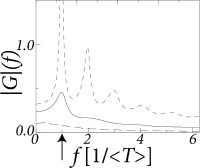
The frequency-dependent gain $\hat{G}$ depends on the filter ${\mathcal{L}}(s)$ which in turns depends on the width of the interval distribution $P_{0}(s)$ (Fig. 14.9B and A, respectively). In Fig. 14.9C we have plotted the signal gain $\hat{G}(\omega)$ for integrate-and-fire neurons with escape noise at different noise levels. At low noise, the signal gain exhibits resonances at the frequency that corresponds to the inverse of the mean interval and multiples thereof. Increasing the noise level, however, lowers the signal gain of the system. For high noise (long-dashed line in Fig. 14.9C) the signal gain at 1000 Hz is ten times lower than the gain at zero frequency. The cut-off frequency depends on the noise level. The gain at zero frequency corresponds to the slope of the gain function $g_{\sigma}(I_{0})$ and changes with the level of noise.

Fig. 14.9: Response properties of a population of leaky integrate-and-fire neurons with escape noise. A. Interval distribution for three different noise levels. The escape rate has been taken as piecewise linear $\rho=\rho_{0}\,[u-\vartheta]{\mathcal{H}}(u-\vartheta)$ . The value of the bias current $I_{0}$ has been adjusted so that the mean interval is always $\langle T\rangle$ =8 ms. B. The corresponding kernel ${\mathcal{L}}^{\rm IF}(x)$ . The dip in the kernel around $x=\langle T\rangle$ is typical for integrate-and-fire neurons. C. Frequency dependent gain $|G(f)|=|\hat{G}(\omega=2\pi f)|$ . Low noise (short dashed line): the sharply peaked interval distribution (standard deviation $0.75$ ms) and rapid fall-off of kernel ${\mathcal{L}}$ lead to a linear response gain $\hat{G}$ with strong resonances at multiples of the intrinsic firing frequency $1/\langle T\rangle$ . High noise (long-dashed line): the broad interval distribution (standard deviation $4$ ms) and broad kernel ${\mathcal{L}}$ suppress resonances in the frequency dependent gain. Medium noise (solid line): A single resonance for an interval distribution with standard deviation $2$ ms. Adapted from (183).

14.3.1 Derivation of the linear response filter (*)

In order to derive the linearized response $\Delta A$ of the population activity to a change in the input we start from the conservation law,

1=\int_{-\infty}^{t}S_{I}(t\,|\,\hat{t})\,A(\hat{t})\,{\text{d}}\hat{t}\,,

(14.48)

cf. Eq. (14.8). As we have seen in Section 14.1 the population equation (14.5) can be obtained by taking the derivative of Eq. (14.8) with respect to $t$ , i.e.,

0={{\text{d}}\over{\text{d}}t}\int_{-\infty}^{t}S_{I}(t\,|\,\hat{t})\,A(\hat{t% })\,{\text{d}}\hat{t}\,.

(14.49)

For constant input $I_{0}$ , the population activity has a constant value $A_{0}$ . We consider a small perturbation of the stationary state, $A(t)=A_{0}+\Delta A(t)$ , that is caused by a small change in the input current, $\Delta I(t)$ . The time-dependent input generates a total postsynaptic potential, $h(t)=h_{0}+\Delta h(t,\hat{t})$ where $h_{0}$ is the postsynaptic potential for constant input $I_{0}$ and

\Delta h(t,\hat{t})=\int_{0}^{b(\hat{t})}\kappa(s)\,\Delta I(t-s)\,{\text{d}}s

(14.50)

is the change of the postsynaptic potential generated by $\Delta I$ . Note that we keep the notation general and include a dependence upon the last firing time $\hat{t}$ . For leaky integrate-and-fire neurons, we set $b(\hat{t})=t-\hat{t}$ whereas for SRM ${}_{0}$ neurons we set $b(\hat{t})=\infty$ . We expand Eq. (14.49) to linear order in $\Delta A$ and $\Delta h$ and find

0={{\text{d}}\over{\text{d}}t}\int_{-\infty}^{t}S_{0}(t-\hat{t})\,\Delta A(% \hat{t})\,{\text{d}}\hat{t}\\ +A_{0}\,{{\text{d}}\over{\text{d}}t}\left\{\int_{-\infty}^{t}{\text{d}}s\,\int% _{-\infty}^{t}{\text{d}}\hat{t}\,\Delta h(s,\hat{t})\,\left.{\partial S_{I}(t% \,|\,\hat{t})\over\partial\Delta h(s,\hat{t})}\right|_{\Delta h=0}\right\}\,.

(14.51)

We have used the notation $S_{0}(t-\hat{t})=S_{I_{0}}(t\,|\,\hat{t})$ for the survivor function of the asynchronous firing state. To take the derivative of the first term in Eq. (14.51) we use ${{\text{d}}}S_{0}(s)/{\text{d}}s=-P_{0}(s)$ and $S_{0}(0)=1$ . This yields

\Delta A(t)=\int_{-\infty}^{t}P_{0}(t-\hat{t})\,\Delta A(\hat{t})\,{\text{d}}% \hat{t}\\ \mbox{}-A_{0}\,{{\text{d}}\over{\text{d}}t}\left\{\int_{-\infty}^{t}{\text{d}}% s\,\int_{-\infty}^{t}{\text{d}}\hat{t}\,\Delta h(s,\hat{t})\,\left.{\partial S% _{I}(t\,|\,\hat{t})\over\partial\Delta h(s,\hat{t})}\right|_{\Delta h=0}\right% \}\,.

(14.52)

We note that the first term on the right-hand side of Eq. (14.52) has the same form as the population integral equation (14.5), except that $P_{0}$ is the interval distribution in the stationary state of asynchronous firing.

To make some progress in the treatment of the second term on the right-hand side of Eq. (14.52), we now restrict the choice of neuron model and focus on either SRM ${}_{0}$ or integrate-and-fire neurons.

(i) For SRM ${}_{0}$ neurons, we may drop the $\hat{t}$ dependence of the potential and set $\Delta h(t,\hat{t})=\Delta h(t)$ where $\Delta h$ is the input potential caused by the time-dependent current $\Delta I$ ; compare Eqs. (14.44) and (14.50). This allows us to pull the variable $\Delta h(s)$ in front of the integral over $\hat{t}$ and write Eq. (14.52) in the form

\Delta A(t)=\int_{-\infty}^{t}P_{0}(t-\hat{t})\,\Delta A(\hat{t})\,{\text{d}}% \hat{t}+A_{0}\,{{\text{d}}\over{\text{d}}t}\int_{0}^{\infty}{\mathcal{L}}(x)\,% \Delta h(t-x)\,{\text{d}}x\,.

(14.53)

with a kernel

{\mathcal{L}}(x)=-\int_{x}^{\infty}d\xi\,{\partial S(\xi|0)\over\partial\Delta h% (\xi-x)}\equiv{\mathcal{L}}^{\rm SRM}(x)\,.

(14.54)

(ii) For leaky integrate-and-fire neurons we set $\Delta h(t,\hat{t})=\Delta h(t)-\Delta h(\hat{t})\,\exp[-(t-\hat{t})/\tau]$ , because of the reinitialization of the membrane potential after the reset (183). After some rearrangements of the terms, Eq. (14.52) becomes identical to Eq. (14.53) with a kernel

{\mathcal{L}}(x)=-\int_{x}^{\infty}d\xi\,{\partial S(\xi|0)\over\partial\Delta h% (\xi-x)}+\int_{0}^{x}d\xi\,e^{-\xi/\tau}\,{\partial S(x|0)\over\partial\Delta h% (\xi)}\equiv{\mathcal{L}}^{\rm IF}(x)\,.

(14.55)

Let us discuss Eq. (14.53). The first term on the right-hand side of Eq. (14.53) is of the same form as the dynamic equation (14.5) and describes how perturbations $\Delta A(\hat{t})$ in the past influence the present activity $\Delta A(t)$ . The second term gives an additional contribution which is proportional to the derivative of a filtered version of the potential $\Delta h$ .

We see from Fig. 14.10 that the width of the kernel ${\mathcal{L}}$ depends on the noise level. For low noise, it is significantly sharper than for high noise.

Fig. 14.10: Interval distribution (A) and the kernel ${\mathcal{L}}^{\rm SRM}(x)$ (B) for SRM ${}_{0}$ neurons with escape noise. The escape rate has been taken as piecewise linear $\rho=\rho_{0}\,[u-\vartheta]{\mathcal{H}}(u-\vartheta)$ . For low noise (solid lines in A and B) the interval distribution is sharply peaked and the kernel ${\mathcal{L}}^{\rm SRM}$ has a small width. For high noise (dashed line) both the interval distribution and the kernel ${\mathcal{L}}^{\rm SRM}$ are broad. The value of the bias current $I_{0}$ has been adjusted so that the mean interval is always 40 ms. The kernel has been normalized to $\int_{0}^{\infty}{\mathcal{L}}(x)\,{\text{d}}x=1$ .

Example: The kernel ${\mathcal{L}}(x)$ for escape noise (*)

In the escape noise model, the survivor function is given by

S_{I}(t\,|\,\hat{t})=\exp\left\{-\int_{\hat{t}}^{t}f[\eta(t^{\prime}-\hat{t})+% h(t^{\prime},\hat{t})]\,{\text{d}}t^{\prime}\right\}

(14.56)

where $f[u]$ is the instantaneous escape rate across the noisy threshold; cf. Chapter 7. We write $h(t,\hat{t})=h_{0}(t-\hat{t})+\Delta h(t,\hat{t})$ . Taking the derivative with respect to $\Delta h$ yields

\left.{\partial S_{I}(t\,|\,\hat{t})\over\partial\Delta h(s,\hat{t})}\right|_{% \Delta h=0}=-{\mathcal{H}}(s-\hat{t})\,{\mathcal{H}}(t-s)\,f^{\prime}[\eta(s-% \hat{t})+h_{0}(s-\hat{t})]\,S_{0}(t-\hat{t})

(14.57)

where $S_{0}(t-\hat{t})=S_{h_{0}}(t\,|\,\hat{t})$ and $f^{\prime}={\text{d}}f(u)/{\text{d}}u$ . For SRM ${}_{0}$ -neurons, we have $h_{0}(t-\hat{t})\equiv h_{0}$ and $\Delta h(t,\hat{t})=\Delta h(t)$ , independent of $\hat{t}$ . The kernel ${\mathcal{L}}$ is therefore

{\mathcal{L}}^{\rm SRM}(t-s)={\mathcal{H}}(t-s)\int_{-\infty}^{s}{\text{d}}% \hat{t}\,f^{\prime}[\eta(s-\hat{t})+h_{0}]\,S_{0}(t-\hat{t})\,.

(14.58)

Example: Absolute refractoriness (*)

Absolute refractoriness is defined by a refractory kernel $\eta(s)=-\infty$ for $0<s<\delta^{\rm abs}$ and zero otherwise. We take an arbitrary escape rate $f(u)\geq 0$ . The only condition on $f$ is that the escape rate goes rapidly to zero for voltages far below threshold: ${\rm lim}_{u\to-\infty}f(u)=0={\rm lim}_{u\to-\infty}f^{\prime}(u)$ .

This yields $f[\eta(t-\hat{t})+h_{0}]=f(h_{0})\,{\mathcal{H}}(t-\hat{t}-\delta^{\rm abs})$ and hence

f^{\prime}[\eta(t-\hat{t})+h_{0}]=f^{\prime}(h_{0})\,{\mathcal{H}}(t-\hat{t}-% \delta^{\rm abs})\,.

(14.59)

The survivor function $S_{0}(s)$ is unity for $s<\delta^{\rm abs}$ and decays as $\exp[-f(h_{0})\,(s-\delta^{\rm abs})]$ for $s>\delta^{\rm abs}$ . Integration of Eq. (14.58) yields

{\mathcal{L}}(t-t_{1})={\mathcal{H}}(t-t_{1}){f^{\prime}(h_{0})\over f(h_{0})}% \exp[-f(h_{0})\,(t-t_{1})]\,.

(14.60)

As we have seen in Section 14.1, absolute refractoriness leads to the Wilson-Cowan integral equation (14.10). Thus ${\mathcal{L}}$ defined in (14.60) is the kernel relating to Eq. (14.10). It could have been derived directly from the linearization of the Wilson-Cowan integral equation (see Exercises). We note that it is a low-pass filter with cut-off frequency $f(h_{0})$ , which depends on the input potential $h_{0}$ .