14.1 Population activity equations
The interval distribution which has already been introduced in Chapter 7 plays a central role in the formulation of the population equation. Before we formulate the evolution of the population activity in terms of this interval distribution , we specify some necessary assumptions. Two key assumptions are that the population is homogeneous and contains non-adaptive neurons so that we can work in the framework of a time-dependent renewal theory. These assumptions will eventually be relaxed in Section 14.1.4 where we extend the theory to the case of a population of adaptive neurons and in Section 14.6 where we treat populations of finite size.
14.1.1 Assumptions of time-dependent renewal theory
In order to formulate a first version of an integral equation for a population of neurons, we start in the framework of time-dependent renewal theory (Chapter 7). To do so, we have to assume the state of a neuron at time to be completely described by (i) its last firing time ; (ii) the input it received for times ; (iii) the characteristics of potential noise sources, be it noise in the input, noise in the neuronal parameters, or noise in the output.
Are these assumptions overly restrictive or can we still place an interesting and rich set of neuron models in the class of models consistent with assumptions (i) - (iii) of time-dependent renewal theory?
The state of a single-variable integrate-and-fire neuron , for example one of the nonlinear integrate-and-fire models of Chapter 5, is completely characterized by its momentary membrane potential . After firing at a time , the membrane potential is reset, so that all information that arrived before the firing is ‘forgotten’. Integration continues with . Therefore knowledge of last firing time and the input current for is sufficient to predict the momentary state of neuron at time and therefore (for a deterministic model) its next firing time. If the integrate-and-fire model is furthermore subject to noise in the form of stochastic spike arrivals of known rate (but unknown spike arrival times), we will not be able to predict the neuron’s exact firing time. Instead we are interested in the probability density
| (14.1) |
that the next spike occurs around time given that the last spike was at time and the neuron was subject to an input for . In practice, it might be difficult to write down an exact analytical formula for for noise models corresponding to stochastic spike arrival or diffusive noise (cf. Chapter 8), but the quantity is still well defined. We call the generalized interval distribution (cf. Chapter 9).
For several other noise models, there exist explicit mathematical expressions for . Consider, for example, integrate-and-fire models with slow noise in the parameters, defined as follows. After each firing time, the value for the reset or the value of the membrane time constant is drawn from a predefined distribution. Between two resets, the membrane potential evolves deterministically. As a consequence, the distribution of the next firing time can be predicted from the distribution of parameters and the deterministic solution of the threshold crossing equations (183). Such a model of slow noise in the parameters can also be considered as an approximation to a heterogeneous population of neurons where different neurons in the population have slightly different, but fixed parameters.
Another tractable noise model is the ‘escape noise’ model which is also the basis for the Generalized Linear Models of spiking neurons already discussed in Chapter 9. The short-term memory approximation SRM of the Spike Response Model with escape noise (cf. Eq. (9.19) in Ch. 9) is a prime example of a model that fits into the framework of renewal theory specified by assumptions (i) - (iii).
The escape noise model can be used in combination with any linear or nonlinear integrate-and-fire model. For a suitable choice of the escape function it provides also an excellent approximation to diffusive noise in the input; cf. Section 9.4 in Ch. 9. An example of how to formulate a nonlinear integrate-and-fire model with escape noise is given below.
The major limitation of time-dependent renewal theory is that, for the moment, we need to exclude adaptation effects, because the momentary state of adaptive neurons not only on the last firing time (and the input in the past) but also on the firing times of earlier spikes. Section 14.1.4 shows that adaptation can be included by extending the renewal theory to a quasi-renewal theory. The treatment of adaptive neurons is important because most cortical neurons exhibit adaptation (Ch. 6).
Example: Escape noise in integrate-and-fire models
Consider an arbitrary (linear or nonlinear) integrate-and-fire model with refractoriness. The neuron has fired its last spike at and enters thereafter an absolute refractory period of time . Integration of the differential equation of the membrane potential ,
| (14.2) |
restarts at time with initial condition . The input current can have an arbitrary temporal structure.
In the absence of noise, the neuron would emit its next spike at the moment when the membrane potential reaches the numerical threshold . In the presence of escape noise, the neuron fires in each short time interval , a spike with probability where
| (14.3) |
is the escape rate which typically depends on the distance between the membrane potential and the threshold, and potentially also on the derivative of the membrane potential; cf. Section 9.4 in Ch. 9.
Knowledge of the input for is sufficient to calculate the membrane potential by integration of Eq. (14.2). The time course of is inserted into Eq. (14.3) to get the instantaneous rate or firing ‘hazard’ for all . By definition, the instantaneous rate vanishes during the absolute refractory time: for . With these notations, we can use the results of Chapter 7 to arrive at the generalized interval distribution
| (14.4) |
Note that, in order to keep notation light, we simply write instead of the more explicit which would emphasize that the hazard depends on the last firing time and the input for ; for the derivation of Eq. 14.4, see also Eq. (7.28) in Ch. 7.
14.1.2 Integral equations for non-adaptive neurons
The integral equation (182; 183; 552) for activity dynamics with time-dependent renewal theory states that the activity at time depends on the fraction of active neurons at earlier times times the probability of observing a spike at given a spike at :
| (14.5) |
Equation (14.5) is easy to understand. The kernel is the probability density that the next spike of a neuron, which is under the influence of an input , occurs at time given that its last spike was at . The number of neurons which have fired at is proportional to and the integral runs over all times in the past. The interval distribution depends on the total input (both the external input and the synaptic input from other neurons in the population). For an unconnected population, corresponds to the external drive. For connected neurons, is the sum of the external input and the recurrent input from other neurons in the population; the case of connected neurons will be further analyzed in Section 14.2.
We emphasize that on the left-hand side of Eq. (14.5) is the expected activity at time while on the right-hand side is the observed activity in the past. In the limit of the number of neurons in the population going to infinity, the fraction of neurons that actually fire in a short time is the same as its expected value . Therefore, Eq. (14.5) becomes exact in the limit of , so that we can use the same symbol for on both sides of the equation. Finite-size effects are discussed in Section 14.6.
We conclude this section with some final remarks on the form of Eq. (14.5). First, we observe that we can multiply the activity value on both sides of the equation with a constant and introduce a new variable . If solves the equation, then will solve it as well. Thus, Eq. (14.5) cannot predict the correct normalization of the activity . This reflects the fact that, instead of defining the activity by a spike count divided by the number of neurons, we could have chosen to work directly with the spike count per unit of time or any other normalization. The proper normalization consistent with our definition of the population activity is derived below in Section 14.1.3.
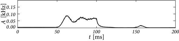
Second, even though Eq. (14.5) is linear in the variable , it is in fact a highly nonlinear equation in the drive, because the kernel depends nonlinearly on the input . However, numerical implementations of the integral-equations lead to rapid schemes that predict the population activity in response to changing input, even in the highly nonlinear regime when strong input transiently synchronizes neurons in the population (Fig. 14.1).
Example: Leaky integrate-and-fire neurons with escape noise
Using appropriate numerical schemes, the integral equation can be used to predict the activity in a homogeneous population of integrate-and-fire neurons subject to a time-dependent input. In each time step, the fraction of neurons that fire is calculated as using (14.5). The value of then becomes part of the observed history and we can evaluate the fraction of neurons in the next time step . For the sake of the implementation, the integral over the past can be truncated at some suitable lower bound (see Section 14.1.5). The numerical integration of Eq. (14.5) predicts well the activity pattern observed in a simulation of 4000 independent leaky integrate-and-fire neurons with exponential escape noise (Fig. 14.1).
|
 |
14.1.3 Normalization and derivation of the integral equation
To derive Eq. (14.5), we recall that is the probability density that a neuron fires at time given its last spike at and an input for . Integration of the probability density over time gives the probability that a neuron which has fired at fires its next spike at some arbitrary time between and . Just as in Chapter 7, we can define a survival probability,
| (14.6) |
i.e., the probability that a neuron which has fired its last spike at “survives” without firing up to time .
We now return to the homogeneous population of neurons in the limit of and assume that the firing of different neurons at time is independent, given that we know the history (the input and last spike) of each neuron. The technical term for such a situation is ’conditional independence’. We consider the network state at time and label all neurons by their last firing time . The proportion of neurons at time which have fired their last spike between and (and have not fired since) is expected to be
| (14.7) |
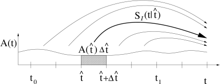
For an interpretation of the integral on the right-hand side of Eq. (14.7), we recall that is the fraction of neurons that have fired in the interval . Of these a fraction are expected to survive from to without firing. Thus among the neurons that we observe at time the proportion of neurons that have fired their last spike between and is expected to be ; cf. Fig. 14.2.
Finally, we use the fact that the total number of neurons remains constant. All neurons have fired at some point in the past.88Neurons which have never fired before are assigned a formal firing time . Thus, if we extend the lower bound of the integral on the right-hand side of Eq. 14.7 to and the upper bound to , the left-hand side becomes equal to one,
| (14.8) |
because all neurons have fired their last spike in the interval . Since the number of neurons remains constant, the normalization of Eq. 14.8 must hold at arbitrary times . Eq. (14.8) is an implicit equation for the population activity and the starting point for the discussions in this and the following chapters.
Since Eq. (14.8) is rather abstract, we will put it into a form that is easier to grasp intuitively. To do so, we take the derivative of Eq. (14.8) with respect to . We find
| (14.9) |
We now use and which is a direct consequence of Eq. (14.6). This yields the activity dynamics of Eq. (14.5).
We repeat an important remark concerning the normalization of the activity. Since Eq. (14.5) is defined as the derivative of Eq. (14.8), the integration constant on the left-hand side of Eq. (14.8) is lost. This is most easily seen for constant activity . In this case the variable can be eliminated on both sides of Eq. (14.5) so that it yields the trivial statement that the interval distribution is normalized to unity. Equation (14.5) is therefore invariant under a rescaling of the activity with any constant , as mentioned earlier. To get the correct normalization of the activity we have to return to Eq. (14.8).
Example: Absolute refractoriness and the Wilson-Cowan integral equation
Let us consider a population of Poisson neurons with an absolute refractory period . A neuron that is not refractory fires stochastically with a rate where is the total input potential caused by an external driving current or synaptic input from other neurons. After firing, a neuron is inactive during a time . The population activity of a homogeneous group of Poisson neurons with absolute refractoriness is (552)
| (14.10) |
Eq. (14.10) represents a special case of Eqs. (14.5) and (14.8) (see Exercises).
The Wilson-Cowan integral equation (14.10) has a simple interpretation. Neurons stimulated by a total postsynaptic potential fire with an instantaneous rate . If there were no refractoriness, we would expect a population activity . However, not all neurons may fire, since some of the neurons are in the absolute refractory period. The fraction of neurons that participate in firing is which explains the factor in curly brackets.
The function in Eq. (14.10) was introduced here as the stochastic intensity of an inhomogeneous Poisson process describing neurons in a homogeneous population. In this interpretation, Eq. (14.10) is the exact equation for the population activity of neurons with absolute refractoriness in the limit of . In their original paper, Wilson and Cowan motivated the function by a distribution of threshold values in an inhomogeneous population. In this case, the population equation (14.10) is only an approximation since correlations are neglected (552).
For constant input potential, , the population activity has a stationary solution (see Fig. 14.3)
| (14.11) |
For the last equality sign we have used the definition of the gain function of Poisson neurons with absolute refractoriness in Eq. (7.50). Equation (14.11) tells us that in a homogeneous population of neurons the population activity in a stationary state is equal to the firing rate of individual neurons, as expected from the discussion in Ch. 12.
Sometimes the stationary solution from Eq. (14.11) is also used in the case of time-dependent input. However, the expression [with from Eq. (14.11)] does not correctly reflect the transients that are seen in the solution of the integral equation (14.10); cf. Fig. 14.3B and Chapter 15.
| A | B |
|---|---|

|
 |
14.1.4 Integral equation for adaptive neurons
The integral equations presented so far are restricted to non-adapting neurons, because we assumed that the knowledge of the input and of the last firing time was sufficient to characterize the state of a neuron. For adapting neurons, however, the whole spiking history can shape the interspike interval distribution. In this section we extend the integral equation (14.5) to the case of adapting neurons.
For an isolated adaptive neuron in the presence of noise, the probability density of firing around time will, in general, depend on its past firing times where denotes the most recent spike time. The central insight is that, in a population of neurons, we can approximate the past firing times by the population activity in the past. Indeed, the probability of one of the neurons having a past spike time in the interval is .
Just as in the time-dependent renewal theory, we will treat the most recent spike of each neuron explicitly. For all spikes with we approximate the actual spike train history of an individual by the average history as summarized in the population activity . Let be the probability of observing a spike at time given the last spike at time , the input-current and the activity history until time , then we can rewrite equation (14.5) in a format suitable for adaptive neurons
| (14.12) |
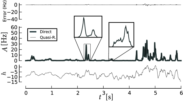
In Section 14.5 we explain the methods to describe populations of adaptive neurons in more detail. Appropriate numerical schemes (Section 14.1.5) make it possible to describe the response of a population of adaptive neurons to arbitrary time-dependent input; see Fig. 14.4.
14.1.5 Numerical methods for integral equations (*)
Integral equations can be solved numerically. However, the type of equation we face in Eq. (14.5) or Eq. (14.12) can not be cast in the typical Volterra or Fredholm forms for which efficient numerical methods have been extensively studied (301; 31). In the following, we describe a method that can be used to solve Eq. (14.5), Eq. (14.12) or Eq. (14.8), but we take as an example the quasi-renewal equivalent of Eq. (14.8)
| (14.13) |
To derive a numerical algorithm, we proceed in three steps. First, truncation of the integral in Eq. (14.13) at some lower bound. Second, the discretization of this integral and, third, the discretization of the integral defining the survivor function. Here we will use the rectangle rule for the discretization of every integral. Note that adaptive quadratures or Monte-Carlo methods could present more efficient alternatives.
The first step is the truncation. The probability to survive a very long time is essentially zero. Let be a period of time such that the survivor is very small. Then, we can truncate the infinite integral in 14.13
| (14.14) |
Next, we proceed to discretize the integral on small bins of size . Let be the vector made of the fraction of neurons at with last spike within and . This definition means that the th element is . The element with is then the momentary population activity in the time step starting at time , , since . Therefore we arrive at
| (14.15) |
Finally, we discretize the integral defining the survival function to obtain as a function of . Because of , we find for sufficiently small time steps
| (14.16) |
Note that we work in a moving coordinate because the index always counts time steps backward starting from the present time . Therefore and refer to the same group of neurons, i.e., those that have fired their last spike around time . Eq. (14.16) indicates that the number of neurons who survive from up to decrease in each time step by an exponential factor. In Eq. (14.16), can be either the renewal conditional intensity of a non-adaptive neuron model (e.g., Eq. (14.3)) or the effective ’quasi-renewal’ intensity of adaptive neurons (see Section 14.5). Together, Eq. (14.15) and (14.16) can be used to solve iteratively.