17.2 Hopfield Model
The Hopfield model (226), consists of a network of neurons, labeled by a lower index , with . Similar to some earlier models (335; 304; 549), neurons in the Hopfield model have only two states. A neuron is ‘ON’ if its state variable takes the value and ‘OFF’ (silent) if . The dynamics evolves in discrete time with time steps . There is no refractoriness and the duration of a time step is typically not specified. If we take ms, we can interpret as an action potential of neuron at time . If we take ms, should rather be interpreted as an episode of high firing rate.
Neurons interact with each other with weights . The input potential of neuron , influenced by the activity of other neurons is
| (17.2) |
The input potential at time influences the probabilistic update of the state variable in the next time step:
| (17.3) |
where is a monotonically increasing gain function with values between zero and one. A common choice is with a parameter . For , we have for and zero otherwise. The dynamics are therefore deterministic and summarized by the update rule
| (17.4) |
For finite the dynamics are stochastic. In the following we assume that in each time step all neurons are updated synchronously (parallel dynamics), but an update scheme where only one neuron is updated per time step is also possible.
The aim of this section is to show that, with a suitable choice of the coupling matrix memory items can be retrieved by the collective dynamics defined in Eq. (17.3), applied to all neurons of the network. In order to illustrate how collective dynamics can lead to meaningful results, we start, in Section 17.2.1, with a detour through the physics of magnetic systems. In Section 17.2.2, the insights from magnetic systems are applied to the case at hand, i.e., memory recall.
| A | B |
|---|---|
|
 |
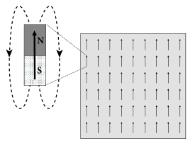
17.2.1 Detour: Magnetic analogy
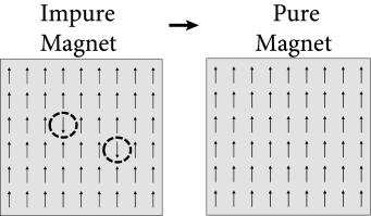
Magnetic material contains atoms which carry a so-called spin. The spin generates a magnetic moment at the microscopic level visualized graphically as an arrow (Fig. 17.5A). At high temperature, the magnetic moments of individual atoms point in all possible directions. Below a critical temperature, however, the magnetic moment of all atoms spontaneously align with each other. As a result, the microscopic effects of all atomic magnetic moments add up and the material exhibits the macroscopic properties of a ferromagnet.
In order to understand how a spontaneous alignment can arise, let us study Eqs. (17.2) and (17.3) in the analogy of magnetic materials. We assume that between all pairs of neurons . and that self-interaction vanishes, .
Each atom is characterized by a spin variable where indicates that the magnetic moment of atom points ‘upward’. Suppose that, at time , all spins take a positive value (), except that of atom which has a value (Fig. 17.5A). We calculate the probability that, at time step , the spin of neuron will switch to . This probability is according to Eq. (17.3)
| (17.5) |
where we have used our assumptions. With and , we find that for any network of more than three atoms, the probability that the magnetic moments of all atoms would align is extremely high. In physical systems, plays the role of an inverse temperature. If becomes small (high temperature), the magnetic moments no longer align and the material loses its spontaneous magnetization.
According to Eq. (17.5) the probability of alignment increases with the network size. This is an artifact of our model with all-to-all interaction between all atoms. Physical interactions, however, rapidly decrease with distance, so that the sum over in Eq. (17.5) should be restricted to the nearest neighbors of neuron , e.g., about 4 to 20 atoms depending on the configuration of the atomic arrangement and the range of the interaction. Interestingly, neurons, in contrast to atoms, are capable of making long-range interactions because of their far-reaching axonal cables and dendritic trees. Therefore, the number of topological neighbors of a given neuron is in the range of thousands.
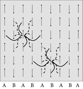
An arrangement of perfectly aligned magnetic elements looks rather boring, but physics offers more interesting examples as well. In some materials, typically consisting of two different types of atoms, say A and B, an anti-ferromagnetic ordering is possible (Fig. 17.6). While one layer of magnetic moments points upward, the next one points downward, so that the macroscopic magnetization is zero. Nevertheless, a highly ordered structure is present. Examples of anti-ferromagnets are some metallic oxides and alloys.
To model an anti-ferromagnet, we choose interactions if and belong to the same class (e.g., both are in a layer of type A or both in a layer of type B), and if one of the two atoms belongs to type A and the other to type B. A simple repetition of the calculation in Eq. (17.5) shows that an anti-ferromagnetic organization of the spins emerges spontaneously at low temperature.
| A | B |
|---|---|
|
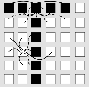 |
The same idea of positive and negative interactions can be used to embed an arbitrary pattern into a network of neurons. Let us draw a pattern of black and white pixels corresponding to active () and inactive () neurons, respectively. The rule extracted from the anti-ferromagnet implies that pixels of opposite color are connected by negative weights, while pixels of the same color have connections with positive weight. This rule can be formalized as
| (17.6) |
This rule forms the basis of the Hopfield model.
17.2.2 Patterns in the Hopfield model
The Hopfield model consists of a network of binary neurons. A neuron is characterized by its state . The state variable is updated according to the dynamics defined in Eq. (17.3).
The task of the network is to store and recall different patterns. Patterns are labeled by the index with . Each pattern is defined as a desired configuration . The network of neurons is said to correctly represent pattern , if the state of all neurons is . In other words, patterns must be fixed points of the dynamics (17.3).
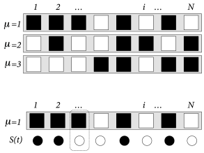
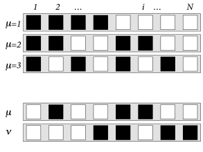
For us as human observers, a meaningful pattern could, for example, be a configuration in form of a ‘T’, such as depicted in Fig. 17.6B. However, visually attractive patterns have large correlations between each other. Moreover, areas in the brain related to memory recall are situated far from the retinal input stage. Since the configuration of neurons in memory-related brain areas is probably very different from those at the retina, patterns in the Hopfield model are chosen as fixed random patterns; cf. Fig. 17.7.
During the set-up phase of the Hopfield network, a random number generator generates, for each pattern a string of independent binary numbers with expectation value . Strings of different patterns are independent. The weights are chosen as
| (17.7) |
with a positive constant . The network has full connectivity. Note that for a single pattern and , Eq. (17.7) is identical to the connections of the anti-ferromagnet, Eq. (17.6). For reasons that become clear later on, the standard choice of the constant is .
| A | B |
|---|---|
|
 |
17.2.3 Pattern retrieval
In many memory retrieval experiments, a cue with partial information is given at the beginning of a recall trial. The retrieval of a memory item is verified by the completion of the missing information.
In order to mimic memory retrieval in the Hopfield model, an input is given by initializing the network in a state . After initialization, the network evolves freely under the dynamics (17.3). Ideally the dynamics should converge to a fixed point corresponding to the pattern which is most similar to the initial state.
In order to measure the similarity between the current state and a pattern , we introduce the overlap (Fig. 17.7B)
| (17.8) |
The overlap takes a maximum value of 1, if , i.e., if the pattern is retrieved. It is close to zero if the current state has no correlation with pattern . The minimum value is achieved if each neuron takes the opposite value to that desired in pattern .
The overlap plays an important role in the analysis of the network dynamics. In fact, using Eq. (17.2) the input potential of a neuron is
| (17.9) |
where we have used Eqs. (17.7) and (17.8). In order to make the results of the calculation independent of the size of the network, it is standard to choose the factor , as mentioned above. In the following we always take unless indicated otherwise. For an in-depth discussion, see the scaling arguments in Chapter 12.
In order to close the argument, we now use the input potential in the dynamics Eq. (17.3) and find
| (17.10) |
Eq. (17.10) highlights that the macroscopic similarity values with completely determine the dynamics of the network.
Example: Memory retrieval
Let us suppose that the initial state has a significant similarity with pattern , e.g., an overlap of and no overlap with the other patterns for .
In the noiseless case Eq. (17.10) simplifies to
| (17.11) |
Hence, each neuron takes, after a single time step, the desired state corresponding to the pattern. In other words, the pattern with the strongest similarity to the input is retrieved, as it should be.
For stochastic neurons we find
| (17.12) |
We note that, given the overlap , the right-hand side of Eq. (17.12) can only take two different values, corresponding to and . Thus, all neurons that should be active in pattern 3 share the same probabilistic update rule
| (17.13) |
Similarly all those that should be inactive share another rule
| (17.14) |
Thus, despite the fact that there are neurons and different patterns, during recall the network breaks up into two macroscopic populations: those that should be active and those that should be inactive. This is the reason why we can expect to arrive at macroscopic population equations, similar to those encountered in part III of the book.
Let us use this insight for the calculation of the overlap at time . We denote the size of the two populations by and , respectively, and find
| (17.15) | |||||
We can interpret the two terms enclosed by the square brackets as the average activity of those neurons that should, or should not, be active, respectively. In the limit of a large network () both groups are very large and of equal size . Therefore, the averages inside the square brackets approach their expectation values. The technical term, used in the physics literature, is that the network dynamics are ‘self-averaging’. Hence, we can evaluate the square brackets with probabilities introduced in Eqs. (17.13) and (17.14). With , we find
| (17.16) |
In the special case that Eq. (17.16) simplifies to an update law
| (17.17) |
where we have replaced by , in order to highlight that updates should be iterated over several time steps.
| A | B |
|---|---|
|
 |
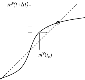
We close with three remarks. First, the dynamics of neurons has been replaced, in a mathematically precise limit, by the iterative update of one single macroscopic variable, i.e., the overlap with one of the patterns. The result is reminiscent of the analysis of the macroscopic population dynamics performed in part III of the book. Indeed, the basic mathematical principles used for the equations of the population activity , are the same as the ones used here for the update of the overlap variable .
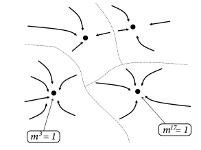
Second, if , the dynamics converges from an initially small overlap to a fixed point with a large overlap, close to one. The graphical solution of the update of pattern (for which a nonzero overlap existed in the initial state) is shown in Fig. 17.8. Because the network dynamics is ‘attracted’ toward a stable fixed point characterized by a large overlap with one of the memorized patterns (Fig. 17.9A), the Hopfield model and variants of it are also called ‘attractor’ networks or ’attractor memories’ (24; 40).
Finally, the assumption that, apart from pattern 3, all other patterns have an initial overlap exactly equal to zero is artificial. For random patterns, we expect a small overlap between arbitrary pairs of patterns. Thus, if the network is exactly in pattern 3 so that , the other patterns have a small but finite overlap , because of spurious correlations between any two random patterns and ; Fig. 17.7B. If the number of patterns is large, the spurious correlations between the patterns can generate problems during memory retrieval, as we will see now.
17.2.4 Memory capacity
How many random patterns can be stored in a network of neurons? Memory retrieval implies pattern completion, starting from a partial cue. An absolutely minimal condition for pattern completion is that at least the dynamics should not move away from the pattern, if the initial cue is identical to the complete pattern (215). In other words, we require that a network with initial state for stays in pattern . Therefore pattern must be a fixed point under the dynamics.
We study a Hopfield network at zero temperature (). We start the calculation as in Eq. 17.9 and insert . This yields
| (17.18) | |||||
where we have separated the pattern from the other patterns. The factor in parenthesis on the right-hand side adds up to one and can therefore be dropped. We now multiply the second term on the right-hand side by a factor . Finally, because , a factor can be pulled out of the argument of the sign-function:
| (17.19) |
The desired fixed point exists only if for all neurons . In other words, even if the network is initialized in perfect agreement with one of the patterns, it can happen that one or a few neurons flip their sign. The probability to move away from the pattern is equal to the probability of finding a value for one of the neurons .
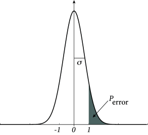
Because patterns are generated from independent random numbers with zero mean, the product is also a binary random number with zero mean. Since the values are chosen independently for each neuron and each pattern , the term can be visualized as a random walk of steps and step size . For a large number of steps, the positive or negative walking distance can be approximated by a Gaussian distribution with zero mean and standard deviation for . The probability that the activity state of neuron erroneously flips is therefore proportional to
| (17.20) |
where we have introduced the error function
| (17.21) |
The most important insight is that the probability of an erroneous state-flip increases with the ratio . Formally, we can define the storage capacity of a network as the maximal number of patterns that a network of neurons can retrieve
| (17.22) |
For the second equality sign we have multiplied both numerator and denominator by a common factor which gives rise to the following interpretation. Since each pattern consists of neurons (i.e., binary numbers), the total number of bits that need to be stored at maximum capacity is . In the Hopfield model, patterns are stored by an appropriate choice of the synaptic connections. The number of available synapses in a fully connected network is . Therefore, the storage capacity measures the number of bits stored per synapse.
Example: Erroneous bits
We can evaluate Eq. (17.20) for various choices of . For example, if we accept an error probability of , we find a storage capacity of .
Hence, a network of 10’000 neurons is able of storing about 1’000 patterns with . Thus in each of the patterns, we expect that about 10 neurons exhibit erroneous activity. We emphasize that the above calculation focuses on the first iteration step only. If we start in the pattern, then about 10 neurons will flip their state in the first iteration. But these flips could in principle cause further neurons to flip in the second iteration and eventually initiate an avalanche of many other changes.
A more precise calculation shows that such an avalanche does not occur, if the number of stored pattern stays below a limit such that (18; 22).
17.2.5 The energy picture
| A | B |
|---|---|
|
 |
The Hopfield model has symmetric interactions . We now show that, in any network with symmetric interactions and asynchronous deterministic dynamics
| (17.23) |
the energy
| (17.24) |
decreases with each state flip of a single neuron (226).
In each time step only one neuron is updated (asynchronous dynamics). Let us assume that after application of Eq. (17.23) neuron has changed its value from at time to while all other neurons keep their value for . The prime indicates values evaluated at time . The change in energy caused by the state flip of neuron is
| (17.25) |
First, because of the update of neuron , we have . Second, because of the symmetry , the two terms on the right-hand side are identical, and . Third, because of Eq. (17.23), the sign of determines the new value of neuron . Therefore the change in energy is . In other words, the energy is a Liapunov function of the deterministic Hopfield network.
Since the dynamics leads to a decrease of the energy, we may wonder whether we can say something about the global or local minimum of the energy. If we insert the definition of the connection weights into the energy function (17.24), we find
| (17.26) |
where we have used the definition of the overlap; cf. Eq. (17.8).
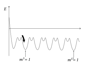
The maximum value of the overlap with a fixed pattern is . Moreover, for random patterns, the correlations between patterns are small. Therefore, if (i.e., recall of pattern ) the overlap with other patterns is . Therefore, the energy landscape can be visualized with multiple minima of the same depth, each minimum corresponding to retrieval of one of the patterns (Fig. 17.9B).
17.2.6 Retrieval of low-activity patterns
There are numerous aspects in which the Hopfield model is rather far from biology. One of these is that in each memory pattern, fifty percent of the neurons are active.
To characterize patterns with a lower level of activity, let us introduce random variables for and with mean . For and we are back to the patterns in the Hopfield model. In the following we are, however, interested in patterns with an activity . To simplify some of the arguments below, we suppose that patterns are generated under the constraint for each , so that all patterns have exactly the same target activity .
The weights in the Hopfield model of Eq. (17.7) are replaced by
| (17.27) |
where is the mean activity of the stored patterns, a constant, and . Note that Eq. (17.7) is a special case of Eq. (17.27) with and .
As before, we work with binary neurons defined by the stochastic update rule in Eqs. (17.2) and (17.3). To analyze pattern retrieval we proceed analogously to Eq. (17.10). Introducing the overlap of low-activity patterns
| (17.28) |
we find
| (17.29) |
Example: Memory retrieval and attractor dynamics
Suppose that at time the overlap with one of the patterns, say pattern 3, is significantly above zero while the overlap with all other patterns vanishes , where denotes the Kronecker-. The initial overlap is . Then the dynamics of the low-activity networks splits up into two groups of neurons, i.e., those that should be ‘ON’ in pattern 3 () and those that should be ‘OFF’ ().
The size of both groups scales with : There are ‘ON’ neurons and ‘OFF’ neurons. For , the population activity of the ‘ON’ group (i.e., the fraction of neurons with state in the ‘ON’ group) is therefore well described by its expectation value
| (17.30) |
Similarly, the ‘OFF’ group has activity
| (17.31) |
To close the argument we determine the overlap at time . Exploiting the split into two groups of size and , respectively, we have
| (17.32) | |||||
Thus, the overlap with pattern 3 has changed from the initial value to a new value . Retrieval of memories works if iteration of Eqs. (17.30) - (17.32) makes converge to a value close to unity while, at the same time, the other overlaps (for ) stay close to zero.
We emphasize that the analysis of the network dynamics presented here does not require symmetric weights but is possible for arbitrary values of the parameter . However, a standard choice is which leads to symmetric weights and to a high memory capacity (522).