2 The Hodgkin-Huxley Model 2.1 Equilibrium potential 2.3 The Zoo of Ion Channels

2.2 Hodgkin-Huxley Model

Hodgkin and Huxley (222) performed experiments on the giant axon of the squid and found three different types of ion current, viz., sodium, potassium, and a leak current that consists mainly of Cl ${}^{-}$ ions. Specific voltage-dependent ion channels, one for sodium and another one for potassium, control the flow of those ions through the cell membrane. The leak current takes care of other channel types which are not described explicitly.

2.2.1 Definition of the model

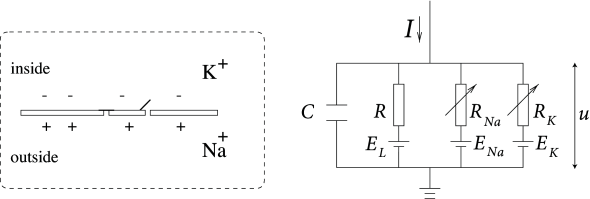
Fig. 2.2: Schematic diagram for the Hodgkin-Huxley model.

The Hodgkin-Huxley model can be understood with the help of Fig. 2.2. The semipermeable cell membrane separates the interior of the cell from the extracellular liquid and acts as a capacitor. If an input current $I(t)$ is injected into the cell, it may add further charge on the capacitor, or leak through the channels in the cell membrane. Each channel type is represented in Fig. 2.2 by a resistor. The unspecific channel has a leak resistance $R$ , the sodium channel a resistance $R_{\rm Na}$ and the potassium channel a resistance $R_{\rm K}$ . The diagonal arrow across the diagram of the resistor indicates that the value of the resistance is not fixed, but changes depending on whether the ion channel is open or closed. Because of active ion transport through the cell membrane, the ion concentration inside the cell is different from that in the extracellular liquid. The Nernst potential generated by the difference in ion concentration is represented by a battery in Fig. 2.2. Since the Nernst potential is different for each ion type, there are separate batteries for sodium, potassium, and the unspecific third channel, with battery voltages $E_{\rm Na},E_{\rm K}$ and $E_{L}$ , respectively.

Let us now translate the above schema of an electrical circuit into mathematical equations. The conservation of electric charge on a piece of membrane implies that the applied current $I(t)$ may be split in a capacitive current $I_{C}$ which charges the capacitor $C$ and further components $I_{k}$ which pass through the ion channels. Thus

I(t)=I_{C}(t)+\sum_{k}I_{k}(t)

(2.3)

where the sum runs over all ion channels. In the standard Hodgkin-Huxley model there are only three types of channel: a sodium channel with index Na, a potassium channel with index K and an unspecific leakage channel with resistance $R$ ; cf. Fig. 2.2. From the definition of a capacity $C=q/u$ where $q$ is a charge and $u$ the voltage across the capacitor, we find the charging current $I_{C}=C\,{\text{d}}u/{\text{d}}t$ . Hence from (2.3)

C{{\text{d}}u\over{\text{d}}t}=-\sum_{k}I_{k}(t)+I(t)\,.

(2.4)

In biological terms, $u$ is the voltage across the membrane and $\sum_{k}I_{k}$ is the sum of the ionic currents which pass through the cell membrane.

Fig. 2.3: The Hodgkin-Huxley model. A. The equilibrium functions for the three variables $m,n,h$ in the Hodgkin-Huxley model. B. The voltage dependent time constant. The resting potential is at $u=-65mV$ (arrow) and parameters are those given in Table 2.1.

As mentioned above, the Hodgkin-Huxley model describes three types of channel. All channels may be characterized by their resistance or, equivalently, by their conductance. The leakage channel is described by a voltage-independent conductance $g_{L}=1/R$ . Since $u$ is the total voltage across the cell membrane and $E_{L}$ the voltage of the battery, the voltage at the leak resistor in Fig. 2.2 is $u-E_{L}$ . Using Ohm’s law, we get a leak current $I_{L}=g_{L}\,(u-E_{L})$ .

The mathematics of the other ion channels is analogous except that their conductance is voltage and time dependent. If all channels are open, they transmit currents with a maximum conductance $g_{\rm Na}$ or $g_{\rm K}$ , respectively. Normally, however, some of the channels are blocked. The breakthrough of Hodgkin and Huxley was that they succeeded to measure how the effective resistance of a channel changes as a function of time and voltage. Moreover, they proposed a mathematical description of their observations. Specifically, they introduced additional ’gating’ variables $m,n$ and $h$ to model the probability that a channel is open at a given moment in time. The combined action of $m$ and $h$ controls the Na ${}^{+}$ channels while the K ${}^{+}$ gates are controlled by $n$ . For example, the effective conductance of sodium channels is modeled as $1/R_{\rm Na}=g_{\rm Na}\,m^{3}\,h$ , where $m$ describes the activation (opening) of the channel and $h$ its inactivation (blocking). The conductance of potassium is $1/R_{\rm K}=g_{\rm K}\,n^{4}$ , where $n$ describes the activation of the channel.

In summary, Hodgkin and Huxley formulated the three ion currents on the right-hand-side of Eq. (2.4) as

\sum_{k}I_{k}=g_{\rm Na}\,m^{3}h\,(u-E_{\rm Na})+g_{\rm K}\,n^{4}\,(u-E_{\rm K% })+g_{L}\,(u-E_{L}).

(2.5)

The parameters $E_{\rm Na}$ , $E_{\rm K}$ , and $E_{L}$ are the reversal potentials.

$x$	$E_{x}\,[{\rm mV}]$	$g_{x}\,[{\rm mS/cm}^{2}]$
${\rm Na}$	55	40
${\rm K}$	-77	35
$L$	-65	0.3

$x$	$\alpha_{x}(u\,/\,\mbox{mV})\,[{\rm ms}^{-1}]$	$\beta_{x}(u\,/\,\mbox{mV})\,[{\rm ms}^{-1}]$
$n$	$0.02(u-25)\,/\,[1-e^{-(u-25)\,/\,9}]$	$-0.002(u-25)\,/\,[1-e^{(u-25)\,/\,9}]$
$m$	$0.182(u+35)\,/\,[1-e^{-(u+35)\,/\,9}]$	$-0.124(u+35)\,/\,[1-e^{(u+35)\,/\,9}]$
$h$	$0.25\;e^{-(u+90)/12}$	$0.25\;e^{(u+62)/6}/e^{(u+90)/12}$

Table 2.1: Parameters for the Hodgkin-Huxley equations fitted on pyramidal neurons of the cortex. The parameters for

n

and

m

were fitted by Zach Mainen (323) on experiments reported by Huguenard et al. (233) and the parameters for

h

by Richard Naud on the experiments reported in Hamill et al. (205). Voltage is measured in mV and the membrane capacity is

C=1\mu\mbox{F/cm}^{2}

The three gating variables $m$ , $n$ , and $h$ evolve according to differential equations of the form

\dot{x}=-{1\over\tau_{x}(u)}[x-x_{0}(u)],

(2.6)

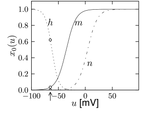
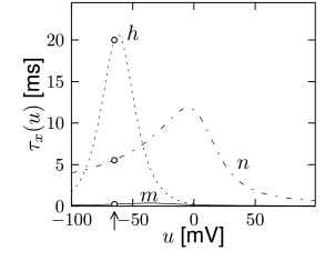
with $\dot{x}={\text{d}}x/{\text{d}}t$ , and where $x$ stands for $m$ , $n$ , or $h$ . The interpretation of Eq. 2.6 is simple: For a fixed voltage $u$ , the variable $x$ approaches the target value $x_{0}(u)$ with a time constant $\tau_{x}(u)$ . The voltage dependence of the time constant and asymptotic value is illustrated in Fig. 2.3. The form of the functions plotted in Fig. 2.3 as well as the maximum conductances and reversal potentials in Eq. (2.5) were deduced by Hodgkin and Huxley from empirical measurements.

Example: Voltage Step

Experimentalists can hold the voltage across the cell membrane at a desired value by injecting an appropriate current into the cell. Suppose that the experimentalist keeps the cell at resting potential $u_{0}=-65$ mV for $t<t_{0}$ and switches the voltage at $t_{0}$ to a new value $u_{1}$ . Integration of the differential equation (2.6) gives, for $t>t_{0}$ , the dynamics

	$\displaystyle m(t)$	$\displaystyle=$	$\displaystyle m_{0}(u_{1})+[m_{0}(u_{0})-m_{0}(u_{1})]\exp\left[{-{(t-t_{0})}% \over{\tau_{m}(u_{1})}}\right],$
	$\displaystyle h(t)$	$\displaystyle=$	$\displaystyle h_{0}(u_{1})+[h_{0}(u_{0})-h_{0}(u_{1})]\exp\left[{-{(t-t_{0})}% \over{\tau_{h}(u_{1})}}\right],$		(2.7)

so that, based on the model with given functions for $m_{0}(u),\,h_{0}(u),\,\tau_{m}(u),\,\tau_{h}(u)$ , we can predict the sodium current $I_{\rm Na}(t)=g_{\rm Na}\,[m(t)^{3}]\,h(t)\,(u_{1}-E_{\rm Na})$ for $t>t_{0}$ generated by voltage step at $t=t_{0}$ .

Similarly, the potassium current caused by a voltage step is $I_{\rm K}(t)=g_{\rm K}\,[n(t)^{4}]\,(u_{1}-E_{\rm K})$ with

n(t)=n_{0}(u_{1})+[n_{0}(u_{0})-n_{0}(u_{1})]\exp\left[{-{(t-t_{0})}\over{\tau% _{n}(u_{1})}}\right].

(2.8)

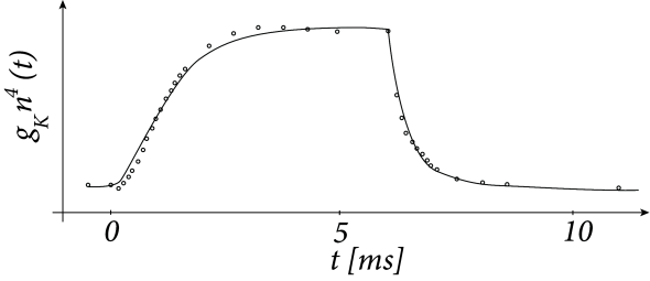
Hodgkin and Huxley used the equations (2.7) and (2.8) to work the other way round. After blocking the sodium channel with appropriate pharmacological agents, they applied a voltage step and measured the time course of the potassium current. Dividing the recorded current through the driving potential $(u_{1}-E_{\rm K})$ yields the time-dependent conductance $g_{\rm K}\,[n(t)^{4}]$ ; cf. Fig. 2.4. Using Eq. (2.8), Hodgkin and Huxley deduced the value of $n_{0}(u_{1})$ and $\tau_{n}(u_{1})$ as well as the exponent of four in $n^{4}(t)$ for potassium. Repeating the experiments for different values $u_{1}$ gives the experimental curves for $n_{0}(u)$ and $\tau_{n}(u)$ .

Fig. 2.4: Original data and fit of Hodgkin and Huxley (1952). The measured time course of the potassium conductance (circles) after application of a voltage step of 25mV (left, marked A) and after return to resting potential (right, B). The fit (solid line) is based on Eq. (2.8). Adapted from (222).

Example: Activation and De-inactivation

The variable $m$ is called an activation variable. To understand this terminology, we note from Fig. 2.3 that the value of $m_{0}(u)$ at the neuronal resting potential of $u$ =-65mV is close to zero. Therefore, at rest, the sodium current $I_{\rm Na}=g_{\rm Na}\,m^{3}h\,(u-E_{\rm Na})$ through the channel vanishes. In other words, the sodium channel is closed.

When the membrane potential increases significantly above the resting potential, the gating variable $m$ increases to its new value $m_{0}(u)$ . As long as $h$ does not change, the sodium current increases and the gate opens. Therefore the variable $m$ ’activates’ the channel. If, after a return of the voltage to rest, $m$ decays back to zero, it is said to be ‘de-activating’.

The terminology of the ‘inactivation’ variable $h$ is analogous. At rest, $h$ has a large positive value. If the voltage increases to a value above -40mV, $h$ approaches a new value $h_{0}(u)$ which is close to rest. Therefore the channel ‘inactivates’ (blocks) with a time constant that is given by $\tau_{h}(u)$ . If the voltage returns to zero, $h$ increases so that the channel undergoes ‘de-inactivation’. This sounds like a tricky vocabulary, but it turns out to be useful to distinguish between a deactivated channel ( $m$ close to zero and $h$ close to one) and an inactivated channel ( $h$ close to zero).

2.2.2 Stochastic Channel Opening

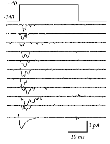
The number of ion channels in a patch of membrane is finite and individual ion channels open and close stochastically. Thus, when an experimentalist records the current flowing through a small patch of membrane, he does not find a smooth and reliable evolution of the measured variable over time but rather a highly fluctuating current, which looks different at each repetition of the experiment (Fig. 2.5).

The Hodgkin-Huxley equations which describe the opening and closing of ion channels with deterministic equations for the variables $m$ , $h$ , and $n$ , correspond to the current density through a hypothetical, extremely large patch of membrane containing an infinite number of channels or, alternatively, to the current through a small patch of membrane but averaged over many repetitions of the same experiment (Fig. 2.5). The stochastic aspects can be included by adding appropriate noise to the model.

Fig. 2.5: Stochastic Channel Activation. The current flowing through a small patch of membrane after application of a voltage step (top row) shows step-like changes and is different in each trial (subsequent traces). Averaging over many trials yields the bottom trace. Adapted from Patlak and Ortiz, 1985 .

Example: Time Constants, Transition Rates, and Channel Kinetics

As an alternative to the formulation of channel gating in Eq. (2.6), the activation and inactivation dynamics of each channel type can also be described in terms of voltage-dependent transition rates $\alpha$ and $\beta$ ,

$\displaystyle\dot{m}=$	$\displaystyle\alpha_{m}(u)\,(1-m)-\beta_{m}(u)\,m$
$\displaystyle\dot{n}=$	$\displaystyle\alpha_{n}(u)\,(1-n)-\beta_{n}(u)\,n$	(2.9)
$\displaystyle\dot{h}=$	$\displaystyle\alpha_{h}(u)\,(1-h)-\beta_{h}(u)\,h.$

The two formulations Eqs. (2.6) and (2.2.2) are equivalent. The asymptotic value $x_{0}(u)$ and the time constant $\tau_{x}(u)$ are given by the transformation $x_{0}(u)=\alpha_{x}(u)/[\alpha_{x}(u)+\beta_{x}(u)]$ and $\tau_{x}(u)=[\alpha_{x}(u)+\beta_{x}(u)]^{-1}$ . The various functions $\alpha$ and $\beta$ , given in Table 2.1, are empirical functions of $u$ that produce the curves in Figure 2.3.

Equations (2.2.2) are typical equations used in chemistry to describe the stochastic dynamics of an activation process with rate constants $\alpha$ and $\beta$ . We may interpret this process as a molecular switch between two states with voltage-dependent transition rates. For example, the activation variable $n$ can be interpreted as the probability of finding a single potassium channel open. Therefore in a patch with $K$ channels, approximately $k\approx(1-n)K$ channels are expected to be closed. We may interpret $\alpha_{n}(u)\Delta t$ as the probability that in a short time interval $\Delta t$ one of the momentarily closed channels switches to the open state.

2.2.3 Dynamics

Fig. 2.6: A. Action potential. The Hodgkin-Huxley model is stimulated by a short, but strong, current pulse between $t=1$ and $t=2$ ms. The time course of the membrane potential $u(t)$ for $t>2$ ms shows the action potential (positive peak) followed by a relative refractory period where the potential is below the resting potential $u_{\rm rest}$ (dashed line). The right panel shows an expanded view of the action potential between $t=2$ and $t=5$ ms. B. The dynamics of gating variables $m$ , $h$ , $n$ illustrate how the action potential is mediated by sodium and potassium channels. C. The sodium current $I_{\rm Na}$ which depends on the variables $m$ and $h$ has a sharp peak during the upswing of an action potential. The potassium current $I_{\rm K}$ is controlled by the variable $n$ and starts with a delay compared to $I_{\rm Na}$ .

In this subsection we study the dynamics of the Hodgkin-Huxley model for different types of input. Pulse input, constant input, step current input, and time-dependent input are considered in turn. These input scenarios have been chosen so as to provide an intuitive understanding of the dynamics of the Hodgkin-Huxley model.

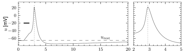
The most important property of the Hodgkin-Huxley model is its ability to generate action potentials. In Fig. 2.6A an action potential has been initiated by a short current pulse of 1 ms duration applied at $t=1$ ms. The spike has an amplitude of nearly 100mV and a width at half maximum of about 2.5ms. After the spike, the membrane potential falls below the resting potential and returns only slowly back to its resting value of -65mV.

Ion channel dynamics during spike generation

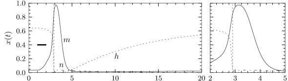
In order to understand the biophysics underlying the generation of an action potential we return to Fig. 2.3A. We find that $m_{0}$ and $n_{0}$ increase with $u$ whereas $h_{0}$ decreases. Thus, if some external input causes the membrane voltage to rise, the conductance of sodium channels increases due to increasing $m$ . As a result, positive sodium ions flow into the cell and raise the membrane potential even further. If this positive feedback is large enough, an action potential is initiated. The explosive increase comes to a natural halt when the membrane potential approaches the reversal potential $E_{\rm Na}$ of the sodium current.

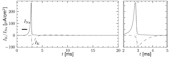
At high values of $u$ the sodium conductance is slowly shut off due to the factor $h$ . As indicated in Fig. 2.3B, the ‘time constant’ $\tau_{h}$ is always larger than $\tau_{m}$ . Thus the variable $h$ which inactivates the channels reacts more slowly to the voltage increase than the variable $m$ which opens the channel. On a similar slow time scale, the potassium (K ${}^{+}$ ) current sets in Fig. 2.6C. Since it is a current in outward direction, it lowers the potential. The overall effect of the sodium and potassium currents is a short action potential followed by a negative overshoot; cf. Fig. 2.6A. The negative overshoot, called hyperpolarizing spike-after potential, is due to the slow de-inactivation of the sodium channel, caused by the $h$ -variable.

Fig. 2.7: A. Spike train of the Hodgkin-Huxley model (with the parameters used in this book) for constant input current $I_{0}$ . B. Gain function. The mean firing rate $\nu$ is plotted as a function of $I_{0}$ . The gain function of the Hodgkin-Huxley model is of type II, because it exhibits a jump. C. Same as A, but for the original parameters found by Hodgkin and Huxley to describe the ion currents in the giant axon of the squid. D. Gain function for the model in C.

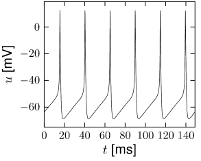
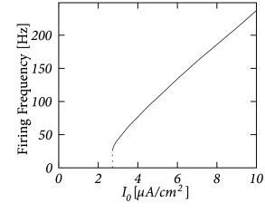
Example: Mean firing rates and gain function

The Hodgkin-Huxley equations (2.4)-(2.2.2) may also be studied for constant input $I(t)=I_{0}$ for $t>0$ . (The input is zero for $t\leq 0$ ). If the value $I_{0}$ is larger than a critical value $I_{\theta}\approx 2.7\mu$ A/cm ${}^{2}$ , we observe regular spiking; Fig. 2.7A. We may define a firing rate $\nu=1/T$ where $T$ is the inter-spike interval.

The firing rate as a function of the constant input $I_{0}$ , often called the ’frequency-current’ relation or ‘f-I-plot’, defines the gain function plotted in Fig. 2.7B. With the parameters given in Table 2.1, the gain function exhibits a jump at $I_{\theta}$ . Gain functions with a discontinuity are called ’type II’.

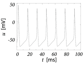
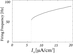
If we shift the curve of the inactivation variable $h$ to more positive voltages, and keep otherwise the same parameters, the modified Hodgkin-Huxley model exhibits a smooth gain function; see Section 2.3.2 and Fig. 2.11. Neuron models or, more generally, ’excitable membranes’ are called ’type I’ or ’class I’ if they have a continuous frequency-current relation. The distinction between excitability of type I and II can be traced back to Hodgkin (223).

Fig. 2.8: A. Spike train of the Hodgkin-Huxley model driven by a time dependent input current. The action potentials occur irregularly. The figure shows the voltage $u$ as a function of time. B. Threshold effect. A short current pulse of 1ms is applied which leads to a excursion of the membrane potential of a few millivolt (dashed line). A slight increase of the strength of the current pulse leads to the generation of an action potential (solid line) with an amplitude of about 100mV above rest (out of bounds).

Example: Stimulation by time-dependent input

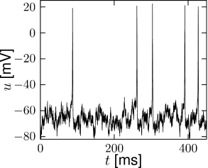
In order to explore a more realistic input scenario, we stimulate the Hodgkin-Huxley model by a time-dependent input current $I(t)$ that is generated by the following procedure. Every 2 ms, a random number is drawn from a Gaussian distribution with zero mean and standard deviation $\sigma=34\mu$ A/cm ${}^{2}$ . To get a continuous input current, a linear interpolation was used between the target values. The resulting time-dependent input current was then applied to the Hodgkin-Huxley model (2.4) - (2.6). The response to the current is the voltage trace shown in Fig. 2.8A. Note that action potentials occur at irregular intervals.

Example: Firing threshold

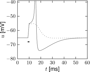
In Fig. 2.8B an action potential (solid line) has been initiated by a short current pulse of 1ms duration. If the amplitude of the stimulating current pulse is reduced below some critical value, the membrane potential (dashed line) returns to the rest value without a large spike-like excursion; cf. Fig. 2.8B. Thus we have a threshold-type behavior.

If we increased the amplitude of the current by a factor of two, but reduced the duration of the current pulse to 0.5ms, so that the current pulse delivers exactly the same electric charge as before, the response curves in 2.8B would look exactly the same. Thus, the threshold of spike initiation can not be defined via the amplitude of the current pulse. Rather, it is the charge delivered by the pulse or, equivalently, the membrane voltage immediately after the pulse, which determines whether an action potential is triggered or not. However, while the notion of a voltage threshold for firing is useful for a qualitative understanding of spike initiation in response to current pulses, it is in itself not sufficient to capture the dynamics of the Hodgkin-Huxley model; see the discussion in this and the next two chapters.

Example: Refractoriness

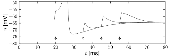
In order to study neuronal refractoriness, we stimulate the Hodgkin-Huxley model by a first current pulse that is sufficiently strong to excite a spike. A second current pulse of the same amplitude as the first one is used to probe the responsiveness of the neuron during the phase of hyperpolarization that follows the action potential. If the second stimulus is not sufficient to trigger another action potential, we have a clear signature of neuronal refractoriness. In the simulation shown in Fig. 2.9, a second spike is not emitted if the second stimulus is given less than 40 milliseconds after the first one. It would, of course, be possible to trigger a second spike after a shorter interval, if a significantly stronger stimulation pulse was used; for classical experiments along those lines, see, e.g. (162).

If we look more closely at the voltage trajectory of Fig. 2.9, we see that neuronal refractoriness manifests itself in two different forms. First, due to the hyperpolarizing spike after-potential the voltage is lower. More stimulation is therefore needed to reach the firing threshold. Second, since a large portion of channels is open immediately after a spike, the resistance of the membrane is reduced compared to the situation at rest. The depolarizing effect of a stimulating current pulse decays therefore faster immediately after the spike than ten milliseconds later. An efficient description of refractoriness plays a major role for simplified neuron models discussed in Chapter 6.

Fig. 2.9: Refractoriness of the Hodgkin-Huxley model. At $t=20$ ms the model is stimulated by a short current pulse (left arrow) so as to trigger an action potential. A second current pulse of the same amplitude applied at $t=35,45$ , or $55$ ms (subsequent arrows) is not sufficient to trigger a second action potential.

Example: Damped Oscillations and Transient Spiking

When stimulated with a small step-increase in current, the Hodgkin-Huxley model with parameters as in Table 2.1 exhibits a damped oscillation with a maximum about 20ms after the onset of the current step; cf. Fig. 2.10. If the step size is large enough, but not sufficient to cause sustained firing, a single spike can be generated. Note that in Fig. 2.10 the input current returns at 200ms to the same value it had a hundred milliseconds before. While the neuron stays quiescent after the first step, it fires a transient spike the second time not because the total input is stronger but because the step starts from a strong negative value.

A spike which is elicited by a step current that starts from a strong negative value and then switches back to zero, would be called a rebound spike. In other words, a rebound spike is triggered by release from inhibition. For example, the Hodgkin-Huxley model with the original parameters for the giant axon of the squid exhibits rebound spikes when a prolonged negative input current is stopped; the model with the set of parameters adopted in this book, however, does not.

The transient spike in Fig. 2.10 occurs about 20 ms after the start of the step. A simple explanation of the transient spike is that the peak of the membrane potential oscillation after the step reaches the voltage threshold for spike initiation, so that a single action potential is triggered. It is indeed the subthreshold oscillations that underly the transient spiking illustrated in Fig. 2.10.

Damped oscillations result from subthreshold inactivation of the sodium current. At rest the sodium currents are not activated ( $m\approx 0$ ) but only partially inactivated ( $h\approx 0.6$ ). Responding to the step stimulus, the membrane potential increases, which activates slightly and de-inactivates slowly the sodium channel. When the input is not strong enough for an action potential to be initiated, the de-inactivation of $I_{\rm Na}$ reduces the effective drive and thus the membrane potential. The system then relaxes to an equilibrium. If, on the other hand, the current was strong enough to elicit a spike, the equilibrium may be reached only after the spike. A further increase in the step current drives sustained firing (Fig. 2.10).