2 The Hodgkin-Huxley Model 2.2 Hodgkin-Huxley Model 2.4 Summary

2.3 The Zoo of Ion Channels

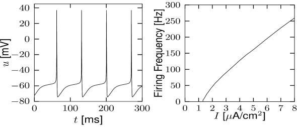
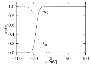
Hodgkin and Huxley used their equations to describe the electro-physiological properties of the giant axon of the squid. These equations capture the essence of spike generation by sodium and potassium ion channels. The basic mechanism of generating action potentials is a short influx of sodium ions that is followed by an efflux of potassium ions. This mechanism of spike generation is essentially preserved in higher organisms, so that with the choice of parameters give in Table 2.1, we have already a first approximate model of neurons in vertebrates. With a further change of parameters we could adapt the model equations to different temperatures so as to account for the fact that neurons at 37 degree Celsius behave differently than neurons in a lab preparation held at a room temperature of 21 degree Celsius.

Fig. 2.10: Damped oscillations and a transient spike. Top. The voltage response to a step current shows a damped oscillation (arrow), a single rebound spike (asterisk) or repetitive firing. Bottom. Time course of the stimulating current.

However, in order to account for the rich biophysics observed in the neurons of the vertebrate nervous system, two types of ion channel are not enough. Neurons come in different types and exhibit different electrical properties which in turn correspond to a large variety of different ion channels. Today, about 200 ion channels are known and many of these have been identified genetically (419). In experimental laboratories where the biophysics and functional role of ion channels is investigated, specific ion channel types can be blocked through pharmacological manipulations. In order to make predictions of blocking results, it is important to develop models that incorporate multiple ion channels. As we will see below (Section 2.3.1), the mathematical framework of the Hodgkin-Huxley model is well suited for such an endeavor.

For other scientific questions, we may only be interested in the firing pattern of neurons and not in the biophysical mechanisms that give rise to it. Later in Part II of this book, we will show that generalized integrate-and-fire models can account for a large variety of neuronal firing patterns (Chapter 6) and predict spike timings of real neurons with high precision (Chapter 11). Therefore, in Part III and IV of the book, where we focus on large networks of neurons, we mainly work with generalized integrate-and-fire rather than biophysical models. Nevertheless, biophysical models, i.e., Hodgkin-Huxley equations with multiple ion channels, serve as an important reference.

2.3.1 Framework for biophysical neuron models

The formalism of the Hodgkin-Huxley equation is extremely powerful, because it enables researchers to incorporate known ion channel types into a given neuron model. Just as before, the electrical properties of a patch of neuronal membrane are described by the conservation of current

C{{\text{d}}u\over{\text{d}}t}=-\sum_{k}I_{k}(t)+I(t)\,,

(2.10)

but in contrast to the simple Hodgkin-Huxley model discussed in the previous section, the right-hand side now contains all types of ion current found in a given neuron. For each ion channel type $k$ , we introduce activation and inactivation variables

I_{k}(t)=g_{k}([Ca^{++}],...)m^{p_{k}}\,h^{q_{k}}\,(u-E_{k}),

(2.11)

where $m$ and $h$ describe activation and inactivation of the channel with equations analogous to Eq. (2.6), $p_{k}$ and $q_{k}$ are empirical parameters, $E_{k}$ is the reversal potential, and $g_{k}$ is the maximum conductance which may depend on secondary variables such as the concentration of calcium, magnesium, dopamine or other substances. In principle, if the dynamics of each channel type (i.e. all parameters that go into Eqs. (2.11) and (2.6) are available, then one needs only to know which channels are present in a given neuron in order to build a biophysical neuron model. Studying the composition of messenger RNA in a drop of liquid extracted from a neuron, gives a strong indication of which ion channel are present in a neuron, and which are not (514). The relative importance of ion channels is not fixed, but depends on the age of neuron as well as other factors. Indeed, a neuron can tune its spiking dynamics by regulating its ion channel composition via a modification of the gene expression profile.

Ion channels are complex transmembrane proteins which exist in many different forms. It is possible to classify an ion channel using (i) its genetic sequence; (ii) the ion type (sodium, potassium, calcium …) that can pass through the open channel; (iii) its voltage dependence; (iv) its sensitivity to second-messengers such as intra-cellular calcium; (v) its presumed functional role; (vi) its response to pharmacological drugs or to neuromodulators such as acetylcholine and dopamine.

Using a notation that mixes the classification schemes (i)-(iii), geneticists have distinguished multiple families of voltage-gated ion channels on the basis of similarities in the amino acid sequences. The channels are labeled with the chemical symbol of the ion of their selectivity, one or two letters denoting a distinct characteristic and a number to determine the sub-family. For instance ‘Kv5’ is the fifth sub-family of the voltage sensitive potassium channel family ‘Kv’. An additional number may be inserted to indicate the channel isoforms, for instance ‘Nav1.1’ is the first isoform that was found within the first subfamily of voltage-dependent sodium channels. Sometimes a lower-case letter is used to point to the splice variants (e.g. ‘Nav1.1a’). Strictly speaking, these names apply to a single cloned gene which corresponds to a channel subunit, whereas the full ion channel is composed of several subunits usually from a given family but possibly from different sub-families.

Traditionally, electrophysiologists have identified channels with subscripts that reflect a combination of the classification schemes (ii)-(vi). The index of the potassium ‘M-current’ $I_{M}$ points to its response to pharmacological stimulation of Muscarinic (M) acetylcholine receptors. Another potassium current, $I_{\rm AHP}$ , shapes the after-hyperpolarization (AHP) of the membrane potential after a spike. Thus the subscript corresponds to the presumed functional role of the channel. Sometimes the functionally characterized current can be related to the genetic classification; for instance $I_{\rm AHP}$ is a calcium-dependent potassium channel associated with the small-conductance ‘SK’ family, but in other cases the link between an electrophysiologically characterized channel and its composition in terms of genetically identified subunits is still uncertain. Linking genetic expression with a functionally characterized ion currents is a fast-expanding field of study (419).

Fig. 2.11: A modification of sodium channel kinetics leads to different neuronal dynamics. A. Response of a model with modified sodium channel to current steps of different amplitudes. B. Delayed spike initiation. A short current pulse of 2 ms duration is applied at $t=8$ ms. The action potential that is elicited in response to the current pulse is shown for decreasing pulse amplitudes ( $I=6.25;5.90;5.88\mu A$ /cm ${}^{2}$ ). Note that the action potential can occur more than 10 ms after the end of the current pulse.

In this section we select a few examples from the zoo of ion channels and illustrate how ion channels can modify the spiking dynamics. The aim is not to quantitatively specify parameters of each ionic current as this depends heavily on the genetic expression of the subunits, cell-type, temperature and neurotransmitters. Rather, we would like to explore qualitatively the influence of ion channel kinetics on neuronal properties. In other words, let us bring the zoo of ion channels to the circus and explore the stunning acts that can be achieved.

2.3.2 Sodium Ion Channels and the Type-I Regime

The parameters of the Hodgkin-Huxley model in Table 2.1 relate to only one type of sodium and potassium ion channel. There are more than 10 different types of sodium channels, each with a slightly different activation and inactivation profile. However, as we will see, even a small change in the ion channel kinetics can profoundly affect the spiking characteristics of a neuron.

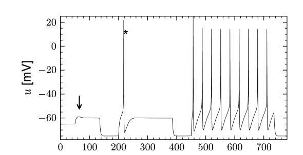
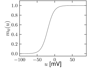
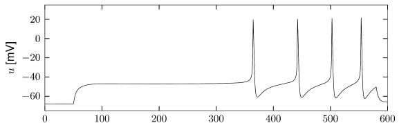
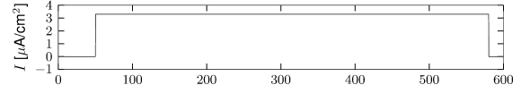
Let us consider a sodium ion channel which has its inactivation curve $h_{0}(u)$ (Fig. 2.3A) shifted to depolarized voltages by 20 mV compared to the parameters in Table 2.1. With maximal conductances $g_{\rm Na}=25$ nS/cm ${}^{2}$ and $g_{\rm K}=40$ nS/cm ${}^{2}$ , the dynamics of a neuron with this modified sodium channel (Fig. 2.11) is qualitatively different from a neuron with the parameters as in Table 2.1 (Figs. 2.7 and 2.10).

Fig. 2.12: Type-I regime with a modified sodium current. A. Regular spiking response to constant input. B. Firing frequency as a function of the constant current.

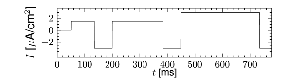
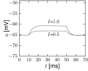
First, the neuron with the modified sodium dynamics shows no damped oscillations in response to a step input (Fig. 2.11A). Second, the neuron responds to a short current pulse which is just slightly above the firing threshold with a delayed action potential (Fig. 2.11B). Third, during regular spiking the shape of the action potential is slightly different in the model with the modified sodium channel (Fig. 2.12A). In particular, the membrane potential between the spikes exhibits an inflection point, unlike the spike train with the original set of parameters (Fig. 2.7A). Finally, the gain function (frequency-current plot) has no gap so that the neuron model can fire at arbitrarily small frequencies (Fig. 2.12B). If we compare this f-I plot with the gain function of the neuron with parameters from Table 2.1, we can distinguish two types of excitability: Type I has a continuous input-output function (Fig. 2.12B), while type II has a discontinuity (Fig. 2.7B).

Fig. 2.13: Spike-frequency adaptation with $I_{\rm M}$ . A. Voltage dependence of the stationary value of the activation variable $m$ and B its time constants for the muscarinic potassium current $I_{\rm M}=g_{M}\,m\,(u-E_{k})$ extracted from experimental observations (562). C. Voltage response to the current shown in D of the original Hodgkin-Huxley model with parameters from Table 2.1 (dashed line) and a model which also contains the $I_{M}$ channel. The model with $I_{M}$ exhibits adaptation. E. Progressive activation of the potassium current $I_{M}$ during the repetitive spiking period shown in C.

2.3.3 Adaptation and Refractoriness

We have seen in Sect. 2.2 that the combination of sodium and potassium channels generates spikes followed by a relative refractory period. The refractoriness is caused by the slow return of the sodium inactivation variable $h$ and the potassium activation variable $n$ to their equilibrium values. The time scale of recovery in the Hodgkin-Huxley model with parameters as in Table 2.1, is 4 ms for the potassium channel activation and 20 ms for the sodium channel inactivation. Other ion channel types, not present in the original Hodgkin-Huxley model, can affect the recovery process on much longer time scales and lead to spike-frequency adaptation: after stimulation with a step current, interspike intervals get successively longer. The basic mechanism of adaptation is the same as that of refractoriness: either a hyperpolarizing current is activated during a spike (and slowly de-activates thereafter) or a depolarizing current is inactivated during a spike and de-inactivates on a much slower time scale.

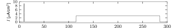
Example: Slow Inactivation of a Hyperpolarizing Current

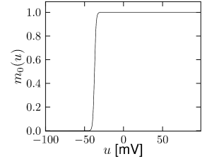
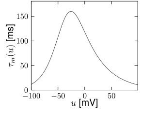
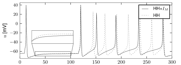
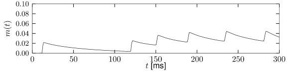
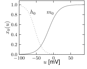
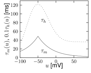
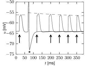
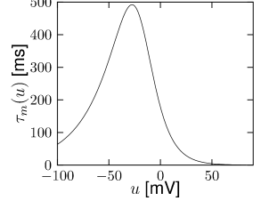
Let us start with the muscarinic potassium channel $I_{M}$ , often called M-current. Genetically, the channel is composed of subunits of the Kv7 family. Figure 2.13A-B shows the activation function as well as the voltage dependence of the time constant as characterized by Yamada et al. [1989]. The activation function (Figure 2.13A) tells us that this channel tends to be activated at voltages above -40 mV and is de-activated below -40 mV with a very sharp transition between the two regimes. Since -40mV is well above the threshold of spike initiation, the membrane potential is never found above -40 mV except during the 1-2 ms of a spike. Therefore the channel partially activates during a spike and, after the end of the action potential, de-activates with a time-constant of 40- 60 ms (Figure 2.13B). The slow deactivation of this potassium channel affects the time course of the membrane potential after a spike. Compared to the original Hodgkin-Huxley model which has only the two currents specified in Table 2.1, a model with an additional $I_{M}$ current exhibits a prolonged hyperpolarizing spike afterpotential and therefore a longer relative refractory period (Figure 2.13C-E).

In the regular firing regime, it is possible that the M-current caused by a previous spike is still partially activated when the next spike is emitted. The partial activation can therefore accumulate over successive spikes. By cumulating over spikes, the activation of $I_{M}$ gradually forces the membrane potential away from the threshold, increasing the interspike interval. This results in a spiking response that appears to ’adapt’ to a step input, hence the name ‘spike-frequency adaptation’ or simply ‘adaptation’ (Figure 2.13C-E).

Fig. 2.14: $I_{\rm A}$ and the refractory period. A. Voltage dependence of the stationary values and (B) time constants of the activation variable $m$ and inactivation variable $h$ for the A-type potassium current $I_{\rm A}=g_{A}\,m\,h\,(u-E_{K})$ extracted from experimental observations in pyramidal neurons of the cortex (276). C. Voltage response to the current shown in D, consisting of a single pulse and a step. E. Progressive activation (solid line) and inactivation (dashed line) of the potassium current $I_{A}$ during the stimulation shown in C and D.

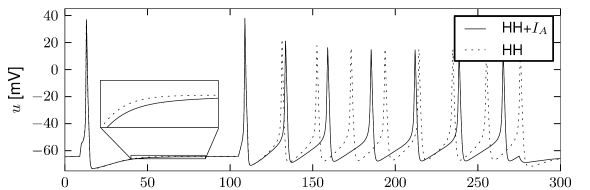
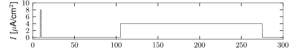
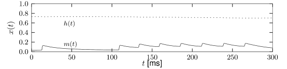
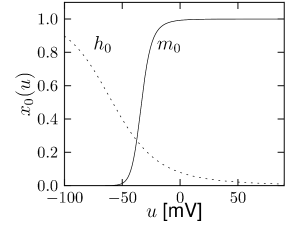
Example: A-current

$I_{A}$ is another potassium ion channel with kinetics similar to $I_{M}$ , but qualitatively different effects: $I_{A}$ makes the relative refractory period longer and stronger without causing much adaptation. To see the distinction between $I_{A}$ and $I_{M}$ , we compare the activation kinetics of both channels (Figure 2.13B and 2.14B). The time constant $\tau_{m}$ of activation is much faster for $I_{A}$ than for $I_{M}$ . This implies that the A-current increases rapidly during the short time of the spike and decays quickly afterward. In other words, the effect of $I_{A}$ is short and strong whereas the effect of $I_{M}$ is long and small. Because the effect of $I_{A}$ does not last as long, it contributes to refractoriness, but only very little to spike frequency adaptation (2.14 C-E). Even though an inactivation process, with variable $h$ , was reported for $I_{A}$ , its time constant $\tau_{h}$ is so long ( $>$ 150ms) that it does not play a role for the above arguments.

Fig. 2.15: Calcium-based spike-frequency adaptation with $I_{\rm K[Ca]}$ and $I_{L}$ . A. Voltage dependence of the stationary values and B time constants of the activation variable $m$ and inactivation variable $h$ of the high-threshold calcium current $I_{\rm HVA}=g_{L}\,h\,m\,(u-E_{Ca})$ extracted from experiments (428). C. Voltage response of a Hodgkin-Huxley model with the calcium current $I_{\rm HVA}$ (dashed line) and a model that also contains a calcium dependent potassium current $I_{\rm K[Ca]}$ . D. External current used for the simulation in C and E. E. Progressive accumulation of intracellular calcium in the two models.

Example: Slow Extrusion of Calcium

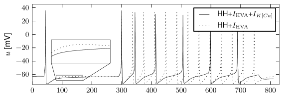
Multiple ion channel families contribute to spike-frequency adaptation. In contrast to the direct action of $I_{M}$ , the calcium dependent potassium channel $I_{\rm K[Ca]}$ generates adaptation indirectly via its dependence on the intracellular calcium concentration. During each spike, calcium enters through the high threshold calcium channel $I_{\rm HVA}$ . As calcium accumulates inside the cell, the calcium dependent potassium channel $I_{\rm K[Ca]}$ gradually opens, lowers the membrane potential, and makes further spike generation more difficult. Thus, the level of adaptation can be read out from the intra-cellular calcium concentration.

In order to understand the accumulation of calcium, we need to discuss the high-threshold calcium channel $I_{\rm HVA}$ . Since it activates above -40 mV to -30 mV, the channel opens during a spike. Its dynamics is therefore similar to that of the sodium current, but the direct effect of $I_{\rm HVA}$ on the shape of the spike is small. Its main role is to deliver a pulse of calcium ions into the neuron. The calcium ions have an important role as second-messengers; they can trigger various cascades of biophysical processes. Intracellular calcium is taken up by internal buffers, or slowly pumped out of the cell, leading to an intricate dynamics dependent on the properties of calcium buffers and calcium pumps. For small calcium transients, however, or when the calcium pump has high calcium affinity and slow extrusion rate, the intracellular calcium dynamics follow (211)

{{\text{d}}[Ca]\over{\text{d}}t}=\phi_{\rm Ca}I_{\rm Ca}+\tau_{\rm Ca}^{-1}% \left([Ca]-[Ca]_{0}\right),

(2.12)

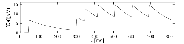
where $[Ca]$ denotes the intracellular calcium concentration, $I_{\rm Ca}$ is the sum of currents coming from all calcium ion channels, $\phi_{Ca}$ is a constant that scales the ionic current to changes in ionic concentration, $[Ca]_{0}$ is a baseline intracellular calcium concentration and $\tau_{\rm Ca}$ is the effective time constant of calcium extrusion. In our simple example the sole source of incoming calcium ions is the high-threshold calcium channel hence $I_{\rm Ca}=I_{\rm HVA}$ . Because of the short duration of the spike, each spike adds a fixed amount of intracellular calcium which afterward decays exponentially (Figure 2.16E), as observed in many cell types (211).

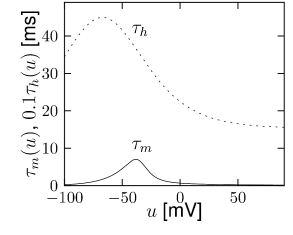
The calcium-dependent potassium channel $I_{\rm K[Ca]}=g_{\rm K[Ca]}\,n\,(u-E_{K})$ is weakly sensitive to the membrane potential but highly sensitive to intra-cellular calcium concentration. The dynamics of activation can be modeled with a calcium dependent time constant (124) of the activation variable $n$

\tau_{n}([Ca])=\frac{k_{3}}{1+k_{2}e^{k_{1}[Ca]}}

(2.13)

and a stationary value (124)

n_{0}=\frac{k_{2}e^{k_{1}[Ca]}}{1+k_{2}e^{k_{1}[Ca]}}

(2.14)

where $k_{1}$ , $k_{2}$ , $k_{3}$ and $g_{\rm K[Ca]}$ are constants.

Figure 2.16 shows the effect of the combined action of calcium channel and $I_{\rm K[Ca]}$ . A single spike generates a transient increase in intracellular calcium which in turn causes a transient increase in $I_{\rm K[Ca]}$ activation which results in a hyperpolarization of the membrane potential compared to a model without $I_{\rm K[Ca]}$ . During sustained stimulation, calcium accumulates over several spikes, so that the effect of $I_{\rm K[Ca]}$ becomes successively larger and interspike intervals increase. The time constant associated with adaptation is a combination of the calcium extrusion time constant and the potassium activation and de-activation time constant.

Fig. 2.16: The persistent sodium channel $I_{\rm NaP}$ increases the firing threshold. A. Activation and inactivation profiles for $I_{\rm NaP}=g_{\rm NaP}\,m\,h\,(u-E_{\rm Na})$ . Activation is fast (a few ms) whereas inactivation is of the order of a second as measured in pyramidal neurons of the cortex (28). B. Slow inactivation affects the effective threshold. In a Hodgkin-Huxley model with persistent sodium current, subthreshold current pulses are injected at different moments (arrows). Only at $t=$ $50ms$ (asterisk), a suprathreshold stimulation was applied. Tuning the strength of the other current pulse so that they are just below spike initiation reveals an effective voltage threshold (dashed line) that is higher immediately after the first spike.

Example: Slow De-inactivation of a Persistent Sodium Channel

The stationary values of activation and inactivation of the persistent sodium channel $I_{\rm NaP}$ (Figure 2.16A) are very similar to that of the normal sodium channel of the Hodgkin-Huxley model. The main difference lies in the time constant. While activation of the channel is quick, it inactivates on a much slower time scale. Hence the name: the current ’persists’. The time constant of the inactivation variable $h$ is of the order of a second.

During sustained stimulation, each spike contributes to the inactivation of the sodium channel and therefore reduces the excitability of the neuron. This special type of refractoriness is not visible in the spike after-potential, but can be illustrated as a relative increase in the effective spiking threshold (Figure 2.16B). Since, after a first spike, the sodium channel is partially inactivated, it becomes more difficult to make the neuron fire a second time.

2.3.4 Subthreshold Effects

Some ion channels have an activation profile $m_{0}(u)$ which has a significant slope well below the spike initiation threshold. During subthreshold activation of the cell by background activity in vivo, or during injection of a fluctuating current, these currents partially activate and inactivate, following the time course of membrane potential fluctuations and shaping them in turn.

We describe two examples of subthreshold ion channel dynamics. The first one illustrates adaptation to a depolarized membrane potential by inactivation of a depolarizing current, which results in a subsequent reduction of the membrane potential. The second example illustrates the opposite behavior: in response to a depolarized membrane potential, a depolarizing current is triggered which increases the membrane potential even further. The two examples therefore correspond to subthreshold adaptation and subthreshold facilitation, respectively.

Example: Subthreshold Adaptation by $I_{h}$

Subthreshold adaptation through a hyperpolarization-activated current $I_{h}$ is present in many cell classes. As the name implies, the current is activated only at hyperpolarized voltages as can be seen in Fig. 2.17A. Thus, the voltage dependence of the activation variable is inverted compared to the normal case and has negative slope. Therefore, the activation variable looks more like an inactivation variable and this is why we choose $h$ as the name of the variable. The channel is essentially closed for prolonged membrane potential fluctuations above -30 mV. The $I_{h}$ current is a nonspecific cation current, meaning that sodium, potassium and calcium can pass through the $I_{h}$ channel when it is open. The reversal potential of this ion channel is usually around -45 mV so that the h-current $I_{h}=g_{h}\,h\,(u-E_{h})$ is depolarizing at resting potential and over most of the subthreshold regime.

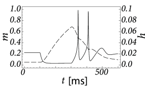
The presence of $I_{h}$ causes the response to step changes in input current to exhibit damped oscillations. The interaction works as follows: suppose an external driving current depolarizes the cell. In the absence of ion channels this would lead to an exponential relaxation to a new value of the membrane potential of, say, -50 mV. Since $I_{h}$ was mildly activated at rest, the membrane potential increase causes the channel to de-activate. The gradual closure of $I_{h}$ removes the effective depolarizing drive and the membrane potential decreases, leading to a damped oscillation (as in Fig. 2.10). This principle can also lead to a rebound spike as seen in Fig. 2.10. Subthreshold adaptation and damped oscillations will be treated in more detail in Chapter 6.

Fig. 2.17: Subthreshold adaptation with $I_{h}$ . A. Stationary values and B. time constants of the variable $h$ controlling the hyperpolarization-activated mixed current $I_{h}$ as measured in pyramidal neurons of the hippocampus (322).

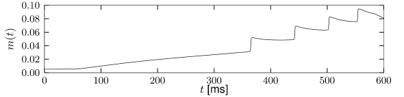
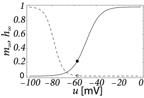
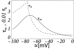
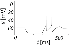
Example: Subthreshold Facilitation by $I_{\rm NaS}$

The sodium ion channel $I_{\rm NaS}$ is slow to activate. Let us consider again stimulation with a step current using a model which contains both the fast sodium current of the Hodgkin-Huxley model and the slow sodium current $I_{\rm NaS}$ . If the strength of the current step is such that it does not activate the fast sodium channel but strong enough to activate $I_{\rm NaS}$ , then the slow activation of this sodium current increases membrane potential gradually with the time constant of activation of the slow sodium current (Fig. 2.18B). The slow depolarization continues until the fast sodium current activates and an action potential is generated (Figure 2.18C). Such delayed spike initiation has been observed in various types of interneurons of the cortex. If the amplitude of the step current is sufficient to immediately activate the fast sodium channels, the gradual activation of $I_{\rm NaS}$ increases the firing frequency leading to spike-frequency facilitation.

Fig. 2.18: Subthreshold facilitation with $I_{\rm NaS}$ . A. Stationary values and B time constants of the activation variable $m$ for the slow sodium current $I_{\rm NaS}$ similar to measurements done in pyramidal neurons of the hippocampus (224). C. Voltage response. D. External Current. E. Slow sodium current activation, leading to delayed spike initiation and firing frequency facilitation.

2.3.5 Calcium spikes and postinhibitory rebound

Postinhibitory rebound means that a hyperpolarizing current, which is suddenly switched off, results in an overshoot of the membrane potential or even in the triggering of one or more action potentials. Through this mechanism, action potentials can be triggered by inhibitory input. These action potentials, however, occur with a certain delay after the arrival of the inhibitory input, viz., after the end of the IPSP (13).

Inactivating currents with a voltage threshold below the resting potential, such as the low-threshold calcium current, can give rise to a much stronger effect of inhibitory rebound than the one seen in the standard Hodgkin-Huxley model. Compared to the sodium current, the low-threshold calcium current $I_{\text{T}}$ has activation and inactivation curves that are shifted significantly toward a hyperpolarized membrane potential so that the channel is completely inactivated ( $h\approx 0$ ) at the resting potential; see Fig. 2.19A and B. In order to open the low-threshold calcium channels it is first of all necessary to remove its inactivation by hyperpolarizing the membrane. The time constant of the inactivation variable $h$ is rather high and it thus takes a while until $h$ has reached a value sufficiently above zero; Fig. 2.19B and D. But even if the channels have been successfully ‘de-inactivated’ they remain in a closed state, because the activation variable $m$ is zero as long as the membrane is hyperpolarized. However, the channels will be transiently opened if the membrane potential is rapidly relaxed from the hyperpolarized level to the resting potential, because activation is faster than inactivation and, thus, there is a short period when both $m$ and $h$ are non-zero. The current that passes through the channels is terminated (‘inactivated’) as soon as the inactivation variable $h$ has dropped to zero again, but this takes a while because of the relatively slow time scale of $\tau_{h}$ . The resulting current pulse is called a low-threshold calcium spike and is much broader than a sodium spike.

The increase in the membrane potential caused by the low-threshold calcium spike may be sufficient to trigger ordinary sodium action potentials. These are the rebound spikes that may occur after a prolonged inhibitory input. Figure 2.19C shows an example of (sodium) rebound spikes that ride on the broad depolarization wave of the calcium spike; note that the whole sequence is triggered at the end of an inhibitory current pulse. Thus release from inhibition causes here a spike-doublet.