9.3 Renewal Approximation of the Spike Response Model

We focus on a Spike Response Model with escape noise; cf. Eqs. (9.1) - (9.3). If the firing rate is low, so that the interspike interval is much longer than the decay time of the refractory kernel $\eta$ , then we can truncate the sum over past firing times and keep track only of the effect of the most recent spike (182)

\displaystyle u(t)=\eta(t-\hat{t})+\int_{0}^{\infty}\kappa(s)\,I^{\rm det}(t-s% )\,{\text{d}}s+u_{\rm rest},

(9.19)

where $\hat{t}$ denotes the last firing time $t^{(f)}<t$ .

Eq. (9.19) is called the ‘short-term memory’ approximation of the SRM and abbreviated as SRM ${}_{0}$ . This model can be efficiently fitted to neural data (251) and will play an important role in Chapter 14 of Part III of this book. In order to emphasize that the value of the membrane potential depends only on the most recent spike, we write in the following $u(t|\hat{t})$ instead of $u(t)$ . Let us summarize the total effect of the input by introducing the ‘input potential’

\displaystyle h(t)=\int_{0}^{\infty}\kappa(s)\,I^{\rm det}(t-s)\,{\text{d}}s

(9.20)

which allows us to rewrite Eq. (9.19) as

\displaystyle u(t|\hat{t})=\eta(t-\hat{t})+h(t)+u_{\rm rest}\,.

(9.21)

The escape rate

\rho(t|\hat{t})=f(u(t|\hat{t}))

(9.22)

depends on the time since the last spike and, implicitly, on the stimulating current $I_{\rm det}(t)$ . Hence $\rho(t|\hat{t})$ is similar to the hazard variable of stationary renewal theory. The arguments of Chapter 7 can be generalized to the case of time-dependent input $I^{\rm det}(t)$ which gives rise to a time-dependent input potential $h(t)$ . Given that the neuron has fired its last spike at time $\hat{t}$ and that we know the input $I^{\rm det}(t^{\prime})$ for $t^{\prime}<t$ we can calculate the probability density that the next spike occurs at time $t>\hat{t}$

P_{I}(t|\hat{t})=\rho(t|\hat{t})\,\exp\left[-\int_{\hat{t}}^{t}\rho(t^{\prime}% |\hat{t})\,{\text{d}}t^{\prime}\right]\,.

(9.23)

Eq. (9.23) generalizes renewal theory to the time-dependent case. Time-dependent renewal theory will play an important role in Chapter 14.

Compared to the standard stationary renewal theory discussed in Chapter 7, there are two important differences. First, the Spike Response Model with escape noise provides a direct path from stationary to time-dependent renewal theory. Second, interval distributions can be linked to refractoriness and vice versa. More precisely, a reduced firing intensity $\rho(t|\hat{t})$ immediately after a spike is an indication that the distance between the membrane potential $u(t|\hat{t})$ and the threshold is increased. The reason can be either a hyperpolarizing spike after-potential $\eta(t)$ or an increase in the firing threshold $\vartheta(t|\hat{t})$ immediately after a spike.

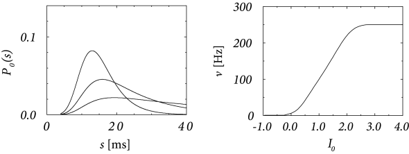
Example: Interval distribution with exponential escape noise

We study a model SRM ${}_{0}$ with membrane potential $u(t|\hat{t})=\eta(t-\hat{t})+h(t)$ and choose a refractory kernel with absolute and relative refractoriness defined as

\eta(s)=\left\{\begin{array}[]{*{2}{c@{\qquad}}c}-\infty\qquad&{\rm for}\qquad% &s<\Delta^{\rm abs}\\ -\eta_{0}\,\exp\left(-{s-\Delta^{\rm abs}\over\tau}\right)\qquad&{\rm for}% \qquad&s>\Delta^{\rm abs}\,.\end{array}\right.

(9.24)

We adopt the exponential escape rate (9.3).

Fig. 9.7 shows the interval distribution for constant input current $I_{0}$ as a function of $s=t-\hat{t}$ . With the normalization $\int_{0}^{\infty}\kappa(s){\text{d}}s=1$ , we have $h_{0}=I_{0}$ . Due to the refractory term $\eta$ , extremely short intervals are impossible and the maximum of the interval distribution occurs at some finite value of $s$ . If $I_{0}$ is increased, the maximum is shifted to the left. The interval distributions of Fig. 9.7A have qualitatively the same shape as those found for cortical neurons. The gain function $\nu=g(I_{0})$ of a noisy SRM ${}_{0}$ neuron is shown in Fig. 9.7B.

We now study the same model with periodic input $I^{\rm det}(t)=I_{0}+I_{1}\cos(\Omega\,t)$ . This leads to an input potential $h(t)=h_{0}+h_{1}\,\cos(\Omega\,t+\varphi_{1})$ with bias $h_{0}=I_{0}$ and a periodic component with a certain amplitude $h_{1}$ and phase $\varphi_{1}$ .

Suppose that a spike has occurred at $\hat{t}=0$ . The probability density that the next spike occurs at time $t$ is given by $P_{I}(t|\hat{t})$ and can be calculated from Eq. (9.23). The result is shown in Fig. 9.8A.

We note that the periodic component of the input is well represented in the response of the neuron. This example illustrates how neurons in the auditory system can transmit stimuli of frequencies higher than the mean firing rate of the neuron. We emphasize that the threshold in Fig. 9.8B is at $\vartheta$ =1. Without noise there would be no output spike. On the other hand, at very high noise levels, the modulation of the interval distribution would be much weaker. Thus a certain amount of noise is beneficial for signal transmission. The existence of an optimal noise level is a phenomenon called stochastic resonance and will be discussed below in Section 9.4.2.