9.1 Escape noise
In the escape noise model, we imagine that an integrate-and-fire neuron with threshold can fire even though the formal threshold has not been reached or may stay quiescent even though the formal threshold has transiently been passed. To do this consistently, we introduce an ‘escape rate’ or ‘firing intensity’ which depends on the momentary state of the neuron.
9.1.1 Escape rate
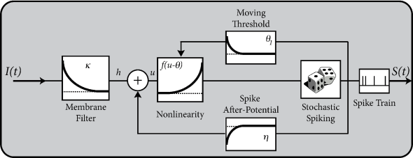
Given the input for and the past firing times , the membrane potential of a generalized integrate-and-fire model (e.g., the adaptive leaky ingrate-and-fire model) or a Spike Response Model (SRM) can be calculated from Eq. (6.7) or Eq. (6.27) respectively; cf. Chapter 6. For example, the value of the membrane potential of a SRM can be expressed as
| (9.1) |
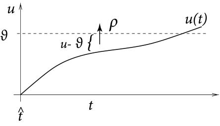
where is the known driving current (the superscript ‘det’ stands for deterministic) and and are filters that describe the response of the membrane to an incoming pulse or an outgoing spike; see Chapter 6. In the deterministic model the next spike occurs when reaches the threshold . In order to introduce some variability into the neuronal spike generator, we replace the strict threshold by a stochastic firing criterion. In the noisy threshold model, spikes can occur at any time with a probability density
| (9.2) |
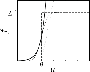
that depends on the momentary distance between the (noiseless) membrane potential and the threshold; see Fig. 9.1. We can think of as an escape rate similar to the one encountered in models of chemical reactions (529). In the mathematical theory of point processes, the quantity is called a ‘stochastic intensity’. Since we use in the context of neuron models we will refer to it as a firing intensity.
The choice of the escape function in Eq. (9.2) is arbitrary. A reasonable condition is to require for so that the neuron does not fire if the membrane potential is far below threshold. A common choice is the exponential,
| (9.3) |
where and are parameters. For , the soft threshold turns into a sharp one so that we return to the noiseless model. Below we discuss some further choices of the escape function in Eq. (9.2).
The SRM of Eq. (9.1) together with the exponential escape rate of Eq. (9.3) is an example of a Generalized Linear Model. Applying the theory of Generalized Linear Models (cf. Chapter 10) to the SRM with escape noise enables a rapid extraction of model parameters from experimental data.
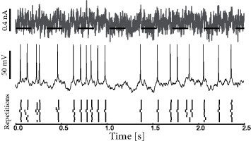
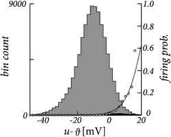
In slice experiments it was found (247) that the exponential escape rate of Eq. (9.3) provides an excellent fit to the spiking intensity of real neurons (Fig. 9.3). Moreover, the firing times of an AdEx model driven by a deterministic fluctuating current and a unknown white noise current can also be well fitted by the Spike Response Model of Eq. (9.1) combined with an exponential escape rate as we will see below in Section 9.4.
Nevertheless, we may wonder whether Eq. (9.2) is a sufficiently general noise model. We have seen in Chapter 2 that the concept of a pure voltage threshold is questionable. More generally, the spike trigger process could, for example, also depend on the slope with which the ‘threshold’ is approached. In the noisy threshold model, we may therefore also consider an escape rate (or hazard) which depends not only on but also on its derivative
| (9.4) |
| A | B |
|---|---|
|
 |
Note that the time-dependence of the firing intensity on the right-hand side of Eq. (9.4) arises implicitly via the membrane potential . In an even more general model, we could in addition include an explicit time dependence, e.g., to account for a reduced spiking probability immediately after a spike at . Instead of an explicit dependence, a slightly more convenient way to implement an additional time dependence is via a time-dependent threshold which we have already encountered in Eq. (6.31). An even more general escape rate model therefore is
| (9.5) |
In Chapter 11 we will see that a Spike Response Model with escape noise and dynamic threshold can explain neuronal firing with a high degree of accuracy.
Example: Bounded versus unbounded escape rate
A stochastic intensity which diverges for such as the exponential escape rate of Eq. (9.3) may seem surprising at a first glance, but it is in fact a necessary requirement for the transition from a soft to a sharp threshold process. Since the escape model has been introduced as a noisy threshold, there should be a limit of low noise that leads us back to the sharp threshold. In order to explore the relation between noisy and deterministic threshold models, we consider as a first step a bounded escape function defined as
| (9.6) |
Thus, the neuron never fires if the voltage is below the threshold. If , the neuron fires stochastically with a rate . Therefore, the mean latency, or expected delay, of a spike is . This implies that the neuron responds slowly and imprecisely, even when the membrane potential is significantly above threshold – and this result looks rather odd. Only in the limit where the parameter goes to zero, the neuron would fire immediately and reliably as soon as the membrane potential crosses the threshold. Thus, a rapid response requires the escape to diverge.
The argument here was based on a step function for the escape rate. A simple choice for a soft threshold which enables a rapid response is a piecewise linear escape rate,
| (9.7) |
with slope for . For , the firing intensity is proportional to ; cf. Fig. 9.4. This corresponds to the intuitive idea that instantaneous firing rates increase with the membrane potential. Variants of the linear escape-rate model are commonly used to describe spike generation in, e.g., auditory nerve fibers (475; 347).
9.1.2 Transition from continuous time to discrete time
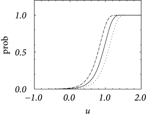
In discrete time, we consider the probability of firing in a finite time step given the neurons has membrane potential . It is bounded from above by one – despite the fact that the escape rate can be arbitrarily large. We start from a model in continuous time and discretize time as it is often done in simulations. In a straightforward discretization scheme, we would calculate the probability of firing during a time step as . However, for , the hazard can take large values; see, e.g., Eq. (9.3). Thus must be taken extremely short so as to guarantee .
In order to arrive at an improved discretization scheme, we calculate the probability that a neuron does not fire in a time step . The probability to survive for a time without firing decays according to . Integration of the differential equation over a finite time yields an exponential factor ; compare the discussion of the survivor function in Chapter 7 (Section 7.5). If the neuron does not survive, it must have fired. Therefore we arrive at a firing probability
| (9.8) |
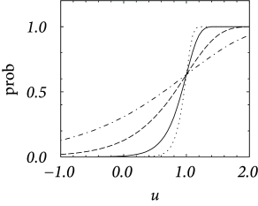
Even if diverges for , the probability of firing remains bounded between zero and one. Aslo, we see that for small , the probability scales as . We see from Fig. 9.5A that, for an exponential escape rate, an increase in the discretization mainly shifts the firing curve to the left while the form remains roughly the same. An increase of the noise level makes the curve flatter; cf. Fig. 9.5B.
Note that, because of refractoriness, it is impossible for integrate-and-fire models (and for real neurons) to fire more than one spike in a short time bin . Refractoriness is implemented in the model of Eq. (9.1) by a significant reset of the membrane potential via the refractory kernel .
| A | B |
|---|---|
|
 |