10 Estimating Models 10 Estimating Models 10.2 Statistical Formulation of Encoding Models

10.1 Parameter optimization in linear and nonlinear models

Before we turn to the statistical formulation of models of encoding and decoding, we need to introduce the language of statistics into neuron modeling. In particular, we will define what is meant by convex problems, optimal solutions, linear models and generalized linear models.

When choosing a neuron model for which we want to estimate the parameters from data, we must satisfy three competing desiderata:

(i) The model must be flexible and powerful enough to fit the observed data. For example, a linear model might be easy to fit, but not powerful enough to account for the data.

(ii) The model must be tractable: we need to be able to fit the model given the modest amount of data available in a physiological recording (preferably using modest computational resources as well); moreover, the model should not be so complex that we cannot assign an intuitive functional role to the inferred parameters.

(iii) The model must respect what is already known about the underlying physiology and anatomy of the system; ideally, we should be able to interpret the model parameters and predictions not only in statistical terms (e.g., confidence intervals, significance tests) but also in biophysical terms (membrane noise, dendritic filtering, etc.). For example, with a purely statistical ‘black box’ model we might be able to make predictions and test their significance, but we will not be able to make links to the biophysics of neurons.

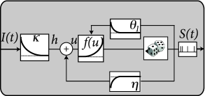
While in general there are many varieties of encoding models that could conceivably satisfy these three conditions, in this chapter we will mainly focus on the SRM with escape noise (Chapter 9). In a more general setting (see Chapter 11), the linear filter can be interpreted not just as local biophysical processes within the neuron, but as a summary of the whole signal processing chain from sensory inputs to the neuron under consideration. In such a general setting, the SRM may also be seen as an example of a ‘generalized linear’ model (GLM) (383; 521). In the following two subsections, we review linear and generalized linear models from the point of view of neuronal dynamics: how is a stimulus $I(t)$ encoded by the neuron?

Fig. 10.1: Measurement of membrane filter. A. Schematic of the linear membrane filter $\kappa$ in discrete time. B. Matrix of temporal inputs (schematic). At each moment in time, the $K$ last time steps of the input current $I_{t}$ serve as an input vector. Rows of the matrix correspond to different input samples.

10.1.1 Linear Models

Let us suppose that an experimentalist injects, with a first electrode, a time-dependent current $I(t)$ in an interval $0<t\leq T$ while recording with a second electrode the membrane voltage $u^{\rm exp}(t)$ . The maximal amplitude of the input current has been chosen small enough for the neuron to stay in the subthreshold regime. We may therefore assume that the voltage is well described by our linear model

u(t)=\int_{0}^{\infty}\kappa(s)I(t-s)\,{\text{d}}s+u_{\rm rest}

(10.1)

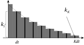
c.f. Section 1.3.5. In order to determine the filter $\kappa$ that describes the linear properties of the experimental neuron, we discretize time in steps of ${\text{d}}t$ and denote the voltage measurement and injected current at time $t$ by $u_{t}^{\rm exp}$ and $I_{t}$ , respectively. Here the time subscript $t\in\mathbb{Z}$ is an integer time step counter. We set $K=s^{\rm max}/{\text{d}}t$ where ${\rm max}(s)\in\mathbb{N}$ and introduce a vector

\mbox{\boldmath\(k\)}=(\kappa({\text{d}}t),\kappa(2{\text{d}}t)\dots,\kappa(K{% \text{d}}t))

(10.2)

which describes the time course $\kappa$ in discrete time; cf. Fig. 10.1A. Similarly, the input current $I$ during the last $k$ time steps is given by the vector.

\mbox{\boldmath\(x\)}_{t}=(I_{t-1},I_{t-2},\dots,I_{t-K})\,{\text{d}}t\,.

(10.3)

The discrete-time version of the integral equation (10.1) is then a simple scalar product

u_{t}=\sum_{l=1}^{K}k_{l}I_{t-l}{\text{d}}t+u_{\rm rest}=\mbox{\boldmath\(k\)}% \cdot\mbox{\boldmath\(x\)}_{t}+u_{\rm rest}\,.

(10.4)

Note that $k$ is the vector of parameters $k_{1},k_{2},\dots k_{K}$ that need to be estimated. In the language of statistics, Eq. 10.4 is a linear model because the observable $u_{t}$ is linear in the parameters. Moreover, $u_{t}$ is a continuous variable so that the problem of estimating the parameters falls in the class of linear regression problems. More generally, regression problems refer to the prediction or modeling of continuous variables whereas classification problems refer to the modeling or prediction of discrete variables.

In order to find a good choice of parameters $k$ , we compare the prediction $u_{t}$ of the model equation (10.4) with the experimental measurement $u_{t}^{\rm exp}$ . In a least-square error approach, the components of the vector $k$ will be chosen such that the squared difference between model voltage and experimental voltage

E(\mbox{\boldmath\(k\)})=\sum_{t=K+1}^{T}[u_{t}^{\rm exp}-u_{t}]^{2}

(10.5)

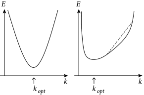
is minimal. An important insight is the following. For any model that is linear in the parameters, the function $E$ in Eq. (10.5) is quadratic and convex in the parameters $k$ of the model. Therefore,

(i) the function $E$ has no non-global local minima as a function of the parameter vector $k$ (in fact, the set of minimizers of $E$ forms a linear subspace in this case, and simple conditions are available to verify that $E$ has a single global minimum, as discussed below);

(ii) the minimum can be found either numerically by gradient descent or analytically by matrix inversion.

While the explicit solution is only possible for linear models, the numerical gradient descent is possible for all kinds of error functions $E$ and yields a unique solution if the error has a unique minimum. In particular, for all error functions which are convex, gradient descent converges to the optimal solution (Fig. 10.2) – and this is what we will exploit in Section 10.2.

Fig. 10.2: Convex function and global minimum. A. A quadratic function (left) and an arbitrary convex function (right). A convex function is curved upward so that any straight line (dashed) connecting two points on the curve stays above the curve. A convex function cannot have a non-global minimum. B. A non-convex function without (left) and with (right) a non-global minimum. Gradient descent refers to a change of the parameter $k$ that leads to a downward move (arrow) on the error surface. In the case on the right, a gradient-descent method can get stuck in the local minimum.

Example: Analytical solution

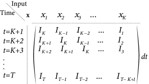
For the analytical solution of the least-square optimization problem, defined by Eqs. (10.4) and (10.5), it is convenient to collect all time points $u_{t}$ , $K+1<t<T$ into a single vector $\mbox{\boldmath$u$}=(u_{K+1},u_{K+2},\dots,u_{T})$ which describes the membrane voltage of the model. Similarly, the observed voltage in the experiment is summarized by the vector $\mbox{\boldmath$u$}^{\rm exp}=(u_{K+1}^{\rm exp},\dots,u_{T}^{\rm exp})$ . Furthermore, let us align the observed input vectors $x$ into a matrix $X$ . More precisely, the matrix has $T-K$ rows consisting of the vector $\mbox{\boldmath$x$}_{t}$ ; cf. Fig. 10.1B. With this notation, Eq. (10.4) can be written as a matrix equation

\mbox{\boldmath\(u\)}=X\,\mbox{\boldmath\(k\)}^{T}+\mbox{\boldmath\(u\)}_{\rm rest}

(10.6)

where $\mbox{\boldmath$u$}_{\rm rest}$ is a vector with all components equal to $u_{\rm rest}$ . We suppose that the value of $u_{\rm rest}$ has already been determined in an earlier experiment.

We search for the minimum of Eq. (10.5), defined by $\nabla_{\mbox{\boldmath$k$}}E=0$ (where $\nabla_{\mbox{\boldmath$k$}}E$ denotes the gradient of $E$ w.r.t. $k$ ), which gives rise a single linear equation for each components of the parameter vector $k$ , i.e., a set of $K$ linear equations. With our matrix notation, the error function is a scalar product

E(\mbox{\boldmath\(k\)})=[\mbox{\boldmath\(u\)}^{\rm exp}-X\,\mbox{\boldmath\(% k\)}-\mbox{\boldmath\(u\)}_{\rm rest}]^{T}\cdot[\mbox{\boldmath\(u\)}^{\rm exp% }-X\,\mbox{\boldmath\(k\)}-\mbox{\boldmath\(u\)}_{\rm rest}]

(10.7)

and the unique solution of the set of linear equations is the parameter vector

\hat{\mbox{\boldmath\(k\)}}_{\rm LS}=(X^{T}X)^{-1}\,X^{T}(\mbox{\boldmath\(u\)% }^{\rm exp}-\mbox{\boldmath\(u\)}_{\rm rest}),

(10.8)

assuming the matrix $(X^{T}X)$ is invertible. (If this matrix is non-invertible, then a unique minimum does not exist.) The subscript highlights that the parameter $\hat{\mbox{\boldmath$k$}}_{\rm LS}$ has been determined by least-square optimization.

10.1.2 Generalized Linear Models

The above linearity arguments work not only in the subthreshold regime, but can be extended to the case of spiking neurons. In the deterministic formulation of the Spike Response Model, the membrane voltage is given

u(t)=\int_{0}^{\infty}\eta(s)S(t-s){\text{d}}s+\int_{0}^{\infty}\kappa(s)I(t-s% )\,{\text{d}}s+u_{\rm rest}\,.

(10.9)

where $S(t)=\sum_{f}\delta(t-t^{(f)})$ is the spike train of the neuron; cf. Eq. (1.22) in Ch. 1 or (9.1) in Ch. 9. Similarly to the passive membrane, the input current enters linearly with a membrane filter $\kappa$ . Similarly, past output spikes $t^{(f)}<t$ enter linearly with a ‘refractory kernel’ or ’adaptation filter’ $\eta$ . Therefore, spike history effects are treated in the SRM as linear contributions to the membrane potential. The time course of the spike history filter $\eta$ can therefore be estimated analogously to that of $\kappa$ .

Regarding the subthreshold voltage, we can generalize Eqs. (10.2) - (10.4). Suppose that the spike history filter $\eta$ extends over a maximum of $J$ time steps. Then we can introduce a new parameter vector

\mbox{\boldmath\(k\)}=(\kappa({\text{d}}t),\kappa(2{\text{d}}t)\dots,\kappa(K{% \text{d}}t),\eta({\text{d}}t),\eta(2{\text{d}}t),\dots,\eta(J{\text{d}}t),u_{% \rm rest})

(10.10)

which includes both the membrane filter $\kappa$ and the spike history filter $\eta$ . The spike train in the last $J$ time steps is represented by the spike count sequence $n_{t-1},n_{t-2},\dots n_{t-J}$ , where $n_{t}\in\{0,1\}$ , and included into the ‘input’ vector

\mbox{\boldmath\(x\)}_{t}=(I_{t-1}{\text{d}}t,I_{t-2}{\text{d}}t,\dots,I_{t-K}% {\text{d}}t,n_{t-1},n_{t-2},\dots n_{t-J},1).\,

(10.11)

The discrete-time version of the voltage equation in the SRM is then again a simple scalar product

u_{t}=\sum_{j=1}^{J}k_{K+j}n_{t-j}+\sum_{k=1}^{K}k_{k}I_{t-k}{\text{d}}t+u_{% \rm rest}=\mbox{\boldmath\(k\)}\cdot\mbox{\boldmath\(x\)}_{t}\,.

(10.12)

Thus, the membrane voltage during the interspike intervals is a linear regression problem that can be solved as before by minimizing the mean square error.

Spiking itself, however, is a nonlinear process. In the SRM with escape rate, the firing intensity is

\rho(t)=f(u(t)-\vartheta)=f(\mbox{\boldmath\(k\)}\cdot\mbox{\boldmath\(x\)}_{t% }-\vartheta)\,,

(10.13)

We have assumed that the firing threshold is constant, but this is no limitation since, in terms of spiking, any dynamic threshold can be included into the spike-history filter $\eta$ .

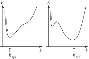
We emphasize that the firing intensity in Eq. (10.13) is a nonlinear function of the parameters $k$ and $b$ which we need to estimate. Nevertheless, rapid parameter estimation is still possible if the function $f$ has properties that we will identify in Section 10.2. The reason is that in each time step firing is stochastic with an instantaneous firing intensity $f$ that only depends on the momentary value of the membrane potential – where the membrane potential can be written as a linear function of the parameters. This insight leads to the notion of Generalized Linear Models (GLM). For a SRM with exponential escape noise $\rho(t)=f(u(t)-\vartheta)=\rho_{0}\exp(u(t)-\vartheta)$ the likelihood of a spike train

\displaystyle L^{n}(\{t^{(1)},t^{(2)},\dots,t^{(n)}\})=\rho(t^{(1)})\cdot\rho(% t^{(2)})\cdot\,\dots\rho(t^{(n)})\,\exp[-\int_{0}^{T}\rho(s){\text{d}}s]\,,

(10.14)

which we have already defined in Chapter 9, Eq. (9.10), is a log-concave function of the parameters (383); i.e., the loglikelihood is a concave function. We will discuss this result in the next section as it is the fundamental reason why parameter optimization for the SRM is computationally efficient (Fig. 10.3).

GLMs are fundamental tools in statistics for which a great deal of theory and computational methods are available. In the following we exploit the elegant mathematical properties of GLMs.