11.1 Encoding Models for Intracellular Recordings
We will focus the discussion on generalized integrate-and-firemodels with escape noise, also called soft-threshold integrate-and-fire models (Fig. 10.3A). The vast majority of studies achieving good predictions of voltage and spike timing use some variant of this model. The reasons lie in the model’s ease of optimization and in its flexibility; cf. Chapter 6. Also, the possibility of casting them into the GLM formalism allows efficient parameter optimization; cf. Chapter 10. In Subsection 11.1.1 we use the SRM as well as soft-threshold integrate-and-fire models to predict the subthreshold voltage of neurons in slices driven by a time-dependent external current. We then use these models to also predict the spike timings of the same neurons (Subsection 11.1.2).
11.1.1 Predicting Membrane Potential
The SRM model describes somatic membrane potential in the presence of an external current (Section 6.4)
| (11.1) |
The parameters of this model define the functional shape of the functions and . Other parameters such as threshold or, in a stochastic model, the sharpness of threshold do not contribute to the mean squared error of the membrane potential as defined in Section 10.3.1. Following the methods of Chapter 10, we can estimate the functions and from recordings of cortical neurons. We note that the spike-afterpotential has units of voltage, whereas the membrane filter has units of resistance over time.
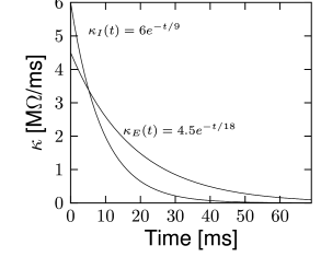
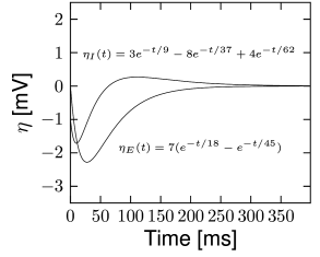
Using in vitro intracellular recordings of cells in layer 2-3 of the somatosensory cortex, Mensi et al. (338) have optimized the functions and on the recorded potential. For both the main type of excitatory neurons and the main type on inhibitory neurons, the membrane filter is well described by a single exponential (Fig. 11.1A). Different cell types have different amplitudes and time constants. The inhibitory neurons are typically faster, with a smaller time constant than the excitatory neurons, suggesting we could discriminate between excitatory and inhibitory neurons in terms of the shape of . Discrimination of cell types, however, is much improved when we take into account the spike-afterpotential. The shape of in inhibitory cells is very different than that in excitatory ones (Fig. 11.1B).
While the spike-afterpotential is a monotonically decreasing function in the excitatory cells, in the inhibitory cells the function is better fitted by two exponentials of opposite polarity. This illustrates that different cell types differ in the functional shape of the spike afterpotential . This finding is consistent with the predictions of Chapter 6 where we discussed the role of different ion channels in shaping . Similar to Fig. 6.14 in Chapter 6, the spike afterpotential of inhibitory neurons is depolarizing 30-150 ms after the spike time, another property providing fast spiking dynamics. Therefore, we conclude that the spike afterpotential of inhibitory neurons has an oscillatory component.
| A | B |
|---|---|
|
 |
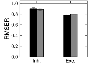
Once the parameters have been extracted from a first set of data, how well does the neuron model predict membrane potential recordings? Qualitatively, we have already seen in Ch. 10 (Fig. 10.5) an example of a typical prediction. Quantitatively, the membrane potential fluctuations of the inhibitory and excitatory neuron have a RMSER (Eq. (10.39)) below one, meaning that the prediction error is smaller than our estimate of the intrinsic error. This indicates that our estimate of the intrinsic error is slightly too large, probably because the actual spike-afterpotential is even longer than a few hundred milliseconds - as we will see below.
Subthreshold mechanisms that can lead to a resonance (Chapter 6) would cause to oscillate in time. Mensi et al. (2012) have tested for the presence of a resonance in and found none. Using two exponentials to model does not improve the prediction of subthreshold membrane potential. Thus, the membrane potential filter is well described by a single exponential with time constant where is the passive membrane resistance and the capacity of the membrane. If we set , we can take the derivative of Eq. (11.1) and write it in the form of a differential equation
| (11.2) |
where is the time course of the net current triggered after a spike.
We have seen in Chapters 2 and 6 that spike-triggered adaptation is mediated by ion channels that change the conductance of the membrane. Biophysics would therefore suggest a spike-triggered change in conductance, such that after every spike the total current that can charge the membrane capacitance is
| (11.3) |
where is the spike triggered change in conductance and its reversal potential. The reversal potential and the time course can be optimized to yield the best goodness-of-fit. In the excitatory neurons, the resulting conductance change follows qualitatively the current-based . The prediction performance, however, is not significantly improved (Fig. 11.2), indicating that describing spike after-effects in terms of potential is a good assumption.
11.1.2 Predicting Spikes
Using the same intracellular recordings as in Fig. 11.1 (338), we now ask whether spike firing can be predicted from the model. The results of the previous subsection provide us with the voltage trajectory of the generalized integrate-and-fire model. Assuming a moving threshold that can undergo a stereotypical change at every spike we can model the conditional firing intensity as (c.f., Eq. (9.27)).
| (11.4) |
Since the parameters regulating were optimized using the subthreshold membrane potential in Section 11.1.1, the only free parameters left are those of the threshold, that is, , and the function . Once the function is expanded in a linear combination of basis functions, maximizing the likelihood (Eq. 10.40) can be done through a convex gradient descent because Eq. 11.4 can be cast into a GLM.
| A | B |
|---|---|
|
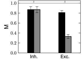 |
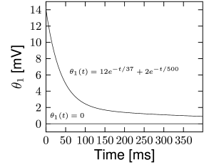
Is the dynamic threshold necessary? Optimizing the parameters on a training dataset, we find no need for moving threshold in the inhibitory neurons (Fig. 11.3A). The threshold in those cells is constant in time. However, the excitatory cells have a strongly moving threshold (Fig. 11.3A) which is characterized by at least two decay time constants. A moving threshold can have several potential biophysical causes. Inactivation of sodium channels is a likely candidate (401) but has not yet been verified by experiments.
How good is the prediction of spike times in inhibitory and excitatory cortical neurons? Qualitatively, the model spike trains resemble the recorded ones with a similar intrinsic variability (Fig. 10.5). Quantitatively, Mensi et al. used the measure of match (see Ch. 10, Eq. (10.52)) and with ms. They found % for the inhibitory neurons and % for the excitatory neurons (Fig. 11.3B). Intuitively, this result means that these models predict more than 80 percent of the ‘predictable’ spikes.
These numbers are averaged over a set of cells. Some cells were predicted better than others such that the reached up to 95% for inhibitory neurons and 87% for excitatory neurons. Similar results are found in excitatory neurons of the layer 5. Spikes from these neurons can be predicted with % on average (407). Other optimization methods but with similar models could improve the spike timing prediction of inhibitory neurons, reaching up to 100% for some cells (267). Thus, the case of inhibitory neurons seems well resolved. The almost perfect match between predicted and experimental spike trains leaves little place for model refinement. Unless the stimulus is specifically designed to probe bursting or post-inhibitory rebound, the generalized integrate-and-fire model is a sufficient description of the fast-spiking inhibitory neuron.
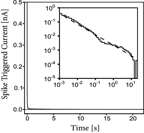
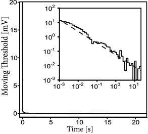
One important feature of the model for spike timing prediction is adaptation. Optimizing a generalized integrate-and-fire model with refractory effects but no adaptation reduces the prediction performance by 20-30% (248), for both the excitatory and inhibitory cortical cells. How long do the effects of spike-triggered adaptation last? Surprisingly, a single spike has a measurable effect more than 10 seconds after the action potential has occurred (Fig 11.4). Thus, adaptation is not characterized by a single time scale (311) and shows up as a power-law decay in both spike-triggered current and threshold (407).
11.1.3 How good are generalized integrate-and-fire models?
For excitatory neurons, a value of % implies that there remains nevertheless 19% of unexplained PSTH variance. Using state-of-the-art model optimization for a full biophysical model with ion channels and extended dendritic tree does not improve the model performance (133). Considering a dependence on the voltage derivative in the escape rate (Chapter 9) can slightly improve the performance (266) but is not sufficient to achieve a flawless prediction. Similarly, taking into account very long spike-history effects (Fig 11.4) and experimental drifts improves mostly the prediction of time-dependent rate performance on long time scales, and only slightly spike time prediction at short timescales (407). Overall, the situation gives the impression that a mechanism might be missing in the generalized integrate-and-fire model and perhaps in the biophysical description as well.
Nevertheless, more than 80 percent of PSTH variance is predicted by generalized soft-threshold integrate-and-fire models during current injection into the soma. This result holds for a time-dependent current which changes on fast as well as slow time scales - a challenging scenario. The effective current driving single neurons in an awake animal in vivo might have comparable characteristics in that it comprises slow fluctuations of the mean as well as fast fluctuations (109; 407). Similarly, the net driving current in connected model networks (see Part III), typically also shows fluctuations around a mean value that changes on a slower time scale. Taken together, generalized integrate-and-fire models are valid models in the physiological input range observed in vivo, and are good candidates for large-scale network simulation and analysis.
Linear dendritic effects show up in the membrane filter and spike-afterpotential; but strongly nonlinear dendrites as observed with multiple recordings from the same neuron (290) can not be accounted for by a generalized soft-threshold integrate-and-fire model or GLM. If nonlinear interactions between different current injection sites along the dendrite are important, a different class of neuron models needs to be considered (Chapter 3).
| A | B |
|---|---|
|
 |