6.4 Spike response model (SRM)
So far, we have described neuronal dynamics in terms of systems of differential equations. There is another approach that was introduced in Section 1.3.5 as the ‘filter picture’. In this picture, the parameters of the model are replaced by (parametric) functions of time, generically called ‘filters’. The neuron model is therefore interpreted in terms of a membrane filter as well as a function describing the shape of the spike (Fig. 6.11) and, potentially, also a function for the time course of the threshold. Together, these three functions establish the Spike Response Model (SRM).
The Spike Response Model is – just like the nonlinear integrate-and-fire models in Chapter 5 or the AdEx in Section 6.1 – a generalization of the leaky integrate-and-fire model. In contrast to nonlinear integrate-and-fire models, the SRM has no ‘intrinsic’ firing threshold but only the sharp numerical threshold for reset. If the nonlinear function of the AdEx is fitted to experimental data, the transition between the linear subthreshold and superthreshold behavior is found to be rather abrupt, so that the nonlinear transition is, for most neurons, well approximated by a sharp threshold (see Fig. 5.3). Therefore, in the SRM, we work with a sharp threshold combined with a linear voltage equation.
While the SRM is therefore somewhat simpler than other models on the level of the spike generation mechanism, the subthreshold behavior of the SRM is richer than that of the integrate-and-fire model discussed so far and can account for various aspects of refractoriness and adaptation. In fact, the SRM combines the most general linear model with a sharp threshold.
It turns out that the integral formulation of the SRM is very useful for data fitting and also the starting point for the Generalized Linear Models in Chapter 9 and 10. Despite the apparent differences between integrate-and-fire models and SRM, the leaky integrate-and-fire model, with or without adaptation variables, is a special case of the SRM. The relation of the SRM to integrate-and-fire models is the topic of Section 6.4.3 – 6.4.4. We now start with a detailed explanation.
6.4.1 Definition of the SRM
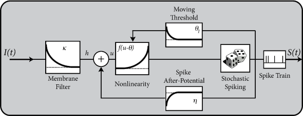
In the framework of the Spike Response Model (SRM) the state of a neuron is described by a single variable which we interpret as the membrane potential. In the absence of input, the variable is at its resting value, . A short current pulse will perturb and it takes some time before returns to rest (Fig. 6.11). The function describes the time course of the voltage response to a short current pulse at time . Because the subthreshold behavior of the membrane potential is taken as linear, the voltage response to an arbitrary time-dependent stimulating current is given by the integral .
Spike firing is defined by a threshold process. If the membrane potential reaches the threshold , an output spike is triggered. The form of the action potential and the after-potential is described by a function . Let us suppose that the neuron has fired some earlier spikes at times . The evolution of is given by
| (6.27) |
The sum runs over all past firing times with of the neuron under consideration. Introducing the spike train , Eq. (6.27) can be also written as a convolution
| (6.28) |
In contrast to the leaky integrate-and-fire neuron discussed in Chapter 1 the threshold is not fixed, but time-dependent
| (6.29) |
Firing occurs whenever the membrane potential reaches the dynamic threshold from below
| (6.30) |
Dynamic thresholds can be directly measured in experiments (162; 35; 338) and are a standard feature of phenomenological neuron models.
Example: Dynamic threshold - and how to get rid of it
A standard model of the dynamic threshold is
| (6.31) |
where is the ‘normal’ threshold of neuron in the absence of spiking. After each output spike, the firing threshold of the neuron is increased by an amount where denote the firing times in the past. For example, during an absolute refractory period , we may set for a few milliseconds to a large and positive value so as to avoid any firing and let it relax back to zero over the next few hundred milliseconds; cf. Fig. 6.12A.
From a formal point of view, there is no need to interpret the variable as the membrane potential. It is, for example, often convenient to transform the variable so as to remove the time-dependence of the threshold. In fact, a general Spike Response Model with arbitrary time-dependent threshold as in Eq. (6.31) can always be transformed into a Spike Response Model with fixed threshold by a change of variables
| (6.32) |
In other words, the dynamic threshold can be absorbed in the definition of the kernel. Note, however, that in this case can no longer be interpreted as the experimentally measured spike after-potential, but must be interpreted as an ‘effective’ spike after-potential.
The argument can also be turned the other way round, so as to remove the spike after-potential and only work with a dynamic threshold; see Fig. 6.12B. However, when an SRM is fitted to experimental data, it is convenient to separate the spike after-effects that are visible in the voltage trace (e.g., in the form of a hyperpolarizing spike-afterpotential, described by the kernel ), from the spike after-effects caused by an increase in the threshold which can be observed only indirectly via the absence of spike firing. Whereas the prediction of spike times is insensitive to the relative contribution of and , the prediction of the subthreshold voltage time course is not. Therefore, it is useful to explicitly work with two distinct adapatation mechanisms in the SRM (338).
| A | B |
|---|---|

|
 |
6.4.2 Interpretation of and
So far Eq. (6.27) in combination with the threshold condition (6.30) defines a mathematical model. Can we give a biological interpretation of the terms?
The kernel is the linear response of the membrane potential to an input current. It describes the time course of a deviation of the membrane potential from its resting value that is caused by a short current pulse (“impulse response”).
The kernel describes the standard form of an action potential of neuron including the negative overshoot which typically follows a spike (the spike afterpotential). Graphically speaking, a contribution is ‘pasted in’ each time the membrane potential reaches the threshold (Fig. 6.12A). Since the form of the spike is always the same, the exact time course of the action potential carries no information. What matters is whether there is the event ‘spike’ or not. The event is fully characterized by the firing time .
In a simplified model, the form of the action potential may therefore be neglected as long as we keep track of the firing times . The kernel describes then simply the ‘reset’ of the membrane potential to a lower value after the spike at just like in the integrate-and-fire model
| (6.33) |
with a parameter . The spike after-potential decays back to zero with a recovery time constant . The leaky integrate-and-fire model is in fact a special case of the SRM, with parameter and .
Example: Refractoriness
Refractoriness may be characterized experimentally by the observation that immediately after a first action potential it is impossible (absolute refractoriness) or more difficult (relative refractoriness) to excite a second spike. In Figure 5.5 (see Chapter 5) we have already seen that refractoriness shows up as increased firing threshold and increased conductance immediately after a spike.
Absolute refractoriness can be incorporated in the SRM by setting the dynamic threshold during a time to an extremely high value that cannot be attained.
Relative refractoriness can be mimicked in various ways. First, after a spike the firing threshold returns only slowly back to its normal value (increase in firing threshold). Second, after the spike the membrane potential, and hence , passes through a regime of hyperpolarization (spike after-potential) where the voltage is below the resting potential. During this phase, more stimulation than usual is needed to drive the membrane potential above threshold. In fact, this is equivalent to a transient increase of the firing threshold (see above).
Third, the responsiveness of the neuron is reduced immediately after a spike. In the SRM we can model the reduced responsiveness by making the shape of and depend on the time since the last spike timing .
We label output spike such that the most recent one receives the label (i.e. ). This means that after each firing event, output spikes need to be relabeled. The advantage, however, is that the last output spike always keeps the label . For simplicity, we often write instead of to denote the most recent spike.
With this notation, a slightly more general version of the Spike Response Model is
| (6.34) |
6.4.3 Mapping the Integrate-and-Fire Model to the SRM
In this section, we show that the leaky integrate-and-fire neuron with adaptation defined above in Eq. (6.7) and (6.8) is a special case of the Spike Response Model. Let us recall that the leaky integrate-and-fire model follows the equation of a linear circuit with resistance and capacity
| (6.35) |
where is the time constant, the leak reversal potential, are adaptation variables, and is the input current to neuron . At each firing time
| (6.36) |
the voltage is reset to a value . At the same time, the adaptation variables are increased by an amount
| (6.37) |
The equations of the adaptive leaky integrate-and-fire model, Eqs. (6.35) and (6.37) can be classified as linear differential equations. However, because of the reset of the membrane potential after firing, the integration is not completely trivial. In fact, there are two different ways of proceeding with the integration. The first method is to treat the reset after each firing as a new initial condition - this is the procedure typically chosen for a numerical integration of the model. Here we follow a different path and describe the reset as a current pulse. As we will see, the result enables a mapping of the leaky integrate-and-fire model to the SRM.
Let us consider a short current pulse applied to the circuit. It removes a charge from the capacitor and lowers the potential by an amount . Thus, a reset of the membrane potential from a value of to a new value corresponds to an ‘output’ current pulse which removes a charge . The reset takes place every time when the neuron fires. The total reset current is therefore
| (6.38) |
where the sum runs over all firing times . We add the output current (6.38) on the right-hand side of (6.35),
| (6.39) | |||||
| (6.40) |
Since Eqs. (6.39) and (6.40) define a system of linear equations, we can integrate each term separately and superimpose the result at the end. To perform the integration, we proceed in three steps. First, we shift the voltage so as to set the equilibrium potential to zero. Second, we calculate the eigenvalues and eigenvectors of the ‘free’ equations in the absence of input (and therefore no spikes). If there are adaptation variables, we have a total of eigenvalues which we label as . The associated eigenvectors are with components . Third, we express the response to an impulse in the voltage (no perturbation in the adaptation variables) in terms of the eigenvectors: . Finally, we express the pulse caused by a reset of voltage and adaptation variables in terms of the eigenvectors .
The response to the reset pulses yields the kernel while the response to voltage pulses yields the filter of the SRM
| (6.41) | |||||
with kernels
| (6.42) | |||||
| (6.43) |
As usual, denotes the Heaviside step function.
| A |
|
| B |
 |
Example: Adaptation and Bursting
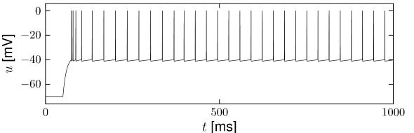
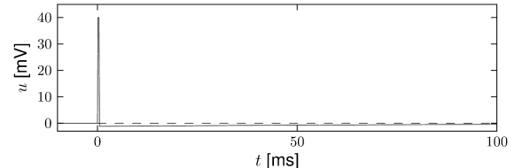
Let us first study a leaky integrate-and-fire model with a single slow adaptation variable which is coupled to the voltage in the subthreshold regime () and increased during spiking by an amount . In this case there are only two equations, one for the voltage and one for adaptation, so that the eigenvectors and eigenvalues can be calculated ‘by hand’. With a parameter , the eigenvalues are and , associated to eigenvectors and . The resulting spike after-potential kernel is shown in Fig. 6.13B. Because of the slow time constant , the kernel has a long hyperpolarizing tail. The neuron model responds to a step current with adaptation, because of accumulation of hyperpolarizing spike-after potentials over many spikes.
As a second example, we consider four adaptation currents with different time constants . We assume pure spike-triggered coupling () so that the integration of the differential equations of gives each an exponential current
| (6.44) |
We choose the time constant of the first current to be very short and (inward current) so as to model the upswing of the action potential (a candidate current would be sodium). A second current (e.g. a fast potassium channel) with a slightly longer time constant is outgoing () and leads to the downswing and rapid reset of the membrane potential. The third current, with a time constant of tens of milliseconds is inward (), while the slowest current is again hyperpolarizing (). Integration of the voltage equation with all four currents generates the spike after-potential shown Fig. 6.14B. Because of the depolarizing spike after-potential induced by the inward current , the neuron model responds to a step current of appropriate amplitude with bursts. The bursts end because of the accumulation of the hyperpolarizing effect of the slowest current.
| A | |
|---|---|

|
|
| B | |

|
6.4.4 Multi-compartment integrate-and-fire model as a SRM (*)
The models discussed in this chapter are point neurons, i.e., models that do not take into account the spatial structure of a real neuron. In Chapter 3 we have already seen that the electrical properties of dendritic trees can be described by compartmental models. In this section, we want to show that neurons with a linear dendritic tree and a voltage threshold for spike firing at the soma can be mapped to the Spike Response Model.
We study an integrate-and-fire model with a passive dendritic tree described by compartments. Membrane resistance, core resistance, and capacity of compartment are denoted by , , and , respectively. The longitudinal core resistance between compartment and a neighboring compartment is ; cf. Fig. 3.8. Compartment represents the soma and is equipped with a simple mechanism for spike generation, i.e., with a threshold criterion as in the standard integrate-and-fire model. The remaining dendritic compartments () are passive.
Each compartment of neuron may receive input from presynaptic neurons. As a result of spike generation, there is an additional reset current at the soma. The membrane potential of compartment is given by
| (6.45) |
where the sum runs over all neighbors of compartment . The Kronecker symbol equals unity if the upper indices are equal; otherwise, it is zero. The subscript is the index of the neuron; the upper indices or refer to compartments. Below we will identify the somatic voltage with the potential of the Spike Response Model.
Equation (6.45) is a system of linear differential equations if the external input current is independent of the membrane potential. The solution of Eq. (6.45) can thus be formulated by means of Green’s functions that describe the impact of an current pulse injected in compartment on the membrane potential of compartment . The solution is of the form
| (6.46) |
Explicit expressions for the Green’s function for arbitrary geometry have been derived by Abbott et al. (1) and Bressloff and Taylor (66).
We consider a network made up of a set of neurons described by Eq. (6.45) and a simple threshold criterion for generating spikes. We assume that each spike of a presynaptic neuron evokes, for , a synaptic current pulse into the postsynaptic neuron . The actual amplitude of the current pulse depends on the strength of the synapse that connects neuron to neuron . The total input to compartment of neuron is thus
| (6.47) |
Here, denotes the set of all neurons that have a synapse with compartment of neuron . The firing times of neuron are denoted by .
In the following we assume that spikes are generated at the soma in the manner of the integrate-and-fire model. That is to say, a spike is triggered as soon as the somatic membrane potential reaches the firing threshold, . After each spike the somatic membrane potential is reset to . This is equivalent to a current pulse
| (6.48) |
so that the overall current due to the firing of action potentials at the soma of neuron amounts to
| (6.49) |
We will refer to equations (6.46)–(6.49) together with the threshold criterion for generating spikes as the multi-compartment integrate-and-fire model.
Using the above specializations for the synaptic input current and the somatic reset current the membrane potential (6.46) of compartment in neuron can be rewritten as
| (6.50) |
with
| (6.51) | ||||
| (6.52) |
The kernel describes the effect of a presynaptic action potential arriving at compartment on the membrane potential of compartment . Similarly, describes the response of compartment to an action potential generated at the soma.
The triggering of action potentials depends on the somatic membrane potential only. We define , and, for , we set . This yields the equation of the SRM
| (6.53) |
| A | B |
|---|---|

|
 |
Example: Two-compartment integrate-and-fire model
We illustrate the methodology by mapping a simple model with two compartments and a reset mechanism at the soma (446) to the Spike Response Model. The two compartments are characterized by a somatic capacitance and a dendritic capacitance . The membrane time constant is and the longitudinal time constant . The neuron fires, if . After each firing the somatic potential is reset to . This is equivalent to a current pulse
| (6.54) |
where is the charge lost during the spike. The dendrite receives spike trains from other neurons and we assume that each spike evokes a current pulse with time course
| (6.55) |
For the two-compartment model it is straightforward to integrate the equations and derive the Green’s function. With the Green’s function we can calculate the response kernels and as defined in Eqs. (6.51) and (6.52). We find
| (6.56) | |||||
with and . Figure 6.15 shows the two response kernels with parameters ms, ms, and . The synaptic time constant is ms. The kernel describes the voltage response of the soma to an input at the dendrite. It shows the typical time course of an excitatory or inhibitory postsynaptic potential. The time course of the kernel is a double exponential and reflects the dynamics of the reset in a two-compartment model.