12.3 Connectivity Schemes
The real connectivity between cortical neurons of different types and different layers, or within groups of neurons of the same type and the same layer is still partially unknown, because experimental data is limited. At most, some plausible estimates of connection probabilities exist. In some cases the connection probability is considered as distance-dependent, in other experimental estimates as uniform in the restricted neighborhood of a cortical column.
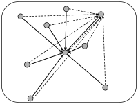
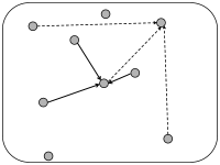
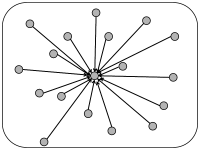
In simulations of spiking neurons, there are a few coupling schemes that are frequently adopted (Fig. 12.6). Most of these assume random connectivity within and between populations. In the following we discuss these schemes with a special focus on the scaling behavior induced by each choice of coupling scheme. Here, scaling behavior refers to a change in the number of neurons that participate in the population.
An understanding of the scaling behavior is important not only for simulations, but also for the mathematical analysis of the network behavior. However, it should be kept in mind that real populations of neurons have a fixed size because, e.g., the number of neurons in a given cortical column is given and, at least in adulthood, does not change dramatically from one day to the next. Typical numbers, counted in one column of mouse somatosensory cortex (barrel cortex, C2) are 5750 excitatory and 750 inhibitory neurons (293). Thus numbers are finite and considerations of the behavior for the number going to infinity are of little relevance to biology.
We note that numbers are even smaller if we break them down per layer. The estimated mean ( standard error of the mean) number of excitatory neurons in each layer (L1 to L6) are as follows: L2, 546 49; L3, 1145 132; L4, 1656 83; L5A, 454 46; L5B, 641 50; L6, 1288 84 and for inhibitory neurons: L1, 26 8; L2, 107 7; L3, 123 19; L4, 140 9; L5A, 90 14; L5B, 131 6; L6, 127 9 (293).
| A | B | C |
|---|---|---|
|
|
|
|
|
 |
Example: Scaling of interaction strength in networks of different sizes
Suppose we simulate a fully connected network of 1 000 noisy spiking neurons. Spikes of each neuron in the population generate in all other neurons an inhibitory input current of strength which lasts for 20 milliseconds. In addition to the inhibitory inputs, each neuron also receives a fixed constant current so that each neurons in the network fires at 5Hz. Since each neuron receives input from itself and from 999 partner neurons, the total rate of inhibitory input is 5kHz. Because each input exerts an effect over 20 milliseconds, a neuron is, at each moment in time, under the influence of about 100 inhibitory inputs - generating a total input .
We now get access to a bigger computer which enables us to simulate a network of 2 000 neurons instead of 1 000. In the new network each neuron therefore receives inhibitory inputs at a rate of 10kHz and is, at each moment in time, under the influence of a total input current . Scaling the synaptic weights by a factor of 1/2 leads us back to the same total input, as before.
Why should we be interested in changing the size of the network? As mentioned before, in biology the network size is fixed. An experimentalist might tell us that the system he studies contains 20 000 neurons, connected with each other with strength (in some arbitrary units) and connection probability of 10%. Running a simulation of the full network of 20 000 neurons is possible, but will take a certain amount of time. We may want to speed up the simulation by simulating a network of 4 000 neurons instead. The question arises whether we should increase the interaction strength in the smaller network compared to the value in the big network.
12.3.1 Full connectivity
The simplest coupling scheme is all-to-all connectivity within a population. All connections have the same strength. If we want to change the number of neurons in the simulation of a population, an appropriate scaling law is
| (12.6) |
This scaling law is a mathematical abstraction that enables us to formally take the limit of while keeping the expected input that a neuron receives from its partners in the population fixed. In the limit of limit, the fluctuations disappear and the expected input can be considered as the actual input to any of the neurons. Of course, real populations are of finite size, so that some fluctuations always remain. But as increases the fluctuations decrease.
A slightly more intricate all-to-all coupling scheme is the following: weights are drawn from a Gaussian distribution with mean and standard deviation . In this case, each neuron in the population sees a somewhat different input, so that fluctuations of the membrane potential are of the order even in the limit of large (146).
| A | B |
|---|---|
|
|
|
|
12.3.2 Random coupling: Fixed coupling probability
Experimentally the probability that a neuron inside a cortical column makes a functional connection to another neuron in the same column is in the range of 10 percent, but varies across layers; cf. Fig. 12.5.
In simulations, we can fix a connection probability and choose connections randomly with probability among all the possible connections. In this case, the number of presynaptic input links to a postsynaptic neuron has a mean value of , but fluctuates between one neuron and the next with variance .
Alternatively, we can take one model neuron after the other and choose randomly presynaptic partners for it (each neuron can be picked only once as a presynaptic partner for a given postsynaptic neuron ). In this case all neurons have, by construction, the same number of input links . By an analogous selection scheme, we could also fix the number of output links to exactly as opposed of simply imposing as the average value.
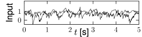
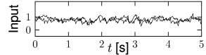
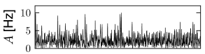
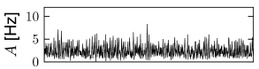
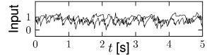
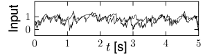
Whatever the exact scheme to construct random connectivity, the number of input connections per neuron increases linearly with the size of the population; see Fig. 12.6B. It is therefore useful to scale the strength of the connections as
| (12.7) |
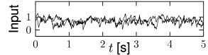
so that the mean input to typical neuron does not change if the number of model neurons in the simulated population is increased. Since in a bigger network individual inputs have less effects with the scaling according to Eq. (12.7), the amount of fluctuations in the input decreases with population size; compare Fig. 12.7.
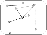
12.3.3 Random coupling: Fixed number of presynaptic partners
The number of synapses onto the dendrites of a single pyramidal neuron is estimated to lie in the range of a few thousand (249). Thus, when one simulates networks of a hundred thousand neurons or millions of neurons, a modeling approach based on a fixed connection probability in the range of 10 percent cannot be correct. Moreover, in an animal participating in an experiment, not all neurons will be active at the same time. Rather only a few subgroups will be active, the composition of which depends on the stimulation conditions and the task. In other words, the number of inputs converging onto a single neuron may be much smaller than a thousand.
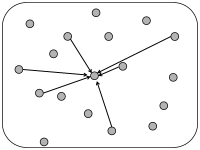
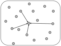
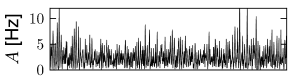
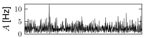
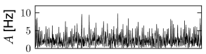
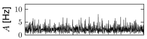
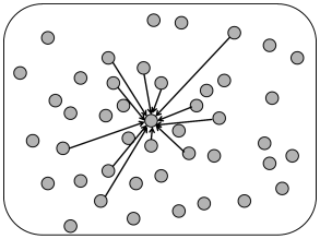
We can construct a random network with a fixed number of inputs by the following procedure. We pick one model neuron after the other and choose randomly its presynaptic partners; see Fig. 12.6C. Whenever the network size is much bigger than , the inputs to a given neuron can be thought of as random samples from the current network activity. No scaling of the connections with the population size is necessary; see Fig. 12.8.
| A | B |
|---|---|
|
|

|
|
12.3.4 Balanced excitation and inhibition
In the simulations of Fig. 12.2, we have assumed a network of excitatory and inhibitory neurons. In other words, our network consists of two interacting populations. The combination of one excitatory and one inhibitory population can be exploited for the scaling of synaptic weights, if the effects of excitation and inhibition are ’balanced’.
In the discussion of scaling in the previous paragraphs, it was mentioned that a fixed connection probability of and a scaling of weights leads to a mean neuronal input current that is insensitive to the size of the simulation; however, fluctuations decrease with increasing . Is there a possibility to work with a fixed connection probability and yet control the size of the fluctuations while changing ?
In a network of two populations, one excitatory and one inhibitory, it is possible to adjust parameters such that the mean input current into a typical neuron vanishes. The condition is that the total amount of excitation and inhibition cancel each other, so that excitation and inhibition are ‘balanced’. The resulting network is called a balanced network or a population with balanced excitation and inhibition (532; 539).
If the network has balanced excitation and inhibition the mean input current to a typical neuron is automatically zero and we do not have to apply a weight rescaling scheme to control the mean. Instead, we can scale synaptic weights so as to control specifically the amount of fluctuations of the input current around zero. An appropriate choice is
| (12.8) |
With this choice, a change in the size of the network hardly affects the mean and variance of the input current into a typical neuron; cf. Fig. 12.9. Note that in simulations of networks of integrate-and-fire neurons, the mean input current to the model neurons is in practice often controlled, and adjusted, through a common constant input to all neurons. In Figs. 12.7 - 12.9 we simply report the main effects of network size on the population activity and synaptic currents; the analysis of the observed phenomena will be postponed to Section 12.4.
| A | B |
|---|---|
|
|
|
|
12.3.5 Interacting Populations
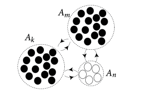
In the previous paragraph we already considered two populations, one of them excitatory and the other one inhibitory. Let us generalize the arguments to a network consisting of several populations; cf. Fig. 12.10. It is convenient to visualize the neurons as being arranged in spatially separate pools, but this is not necessary. All neurons could, for example, be physically localized in the same column of the visual cortex, but of three different types: excitatory, fastspiking inhibitory, and non-fastspiking interneurons.
| A | B |
|---|---|
|
 |
We assume that neurons are homogeneous within each pool. The activity of neurons in pool is
| (12.9) |
where is the number of neurons in pool and denotes the set of neurons that belong to pool . We assume that each neuron in pool receives input from all neurons in pool with strength ; cf. Fig. 12.10. The time course caused by a spike of a presynaptic neuron may depend on the synapse type, i.e., a connection from a neuron in pool to a neuron in pool , but not on the identity of the two neurons. The input current to a neuron in group is generated by the spikes of all neurons in the network,
| (12.10) | |||||
where denotes the time course of a postsynaptic current caused by spike firing at time of the presynaptic neuron which is part of population . We use Eq. (12.9) to replace the sum on the right-hand side of Eq. (12.10) and obtain
| (12.11) |
We have dropped the index since the input current is the same for all neurons in pool .
Thus, we conclude that the interaction between neurons of different pools can be summarized by the population activity of the respective pools. Note that Eq. (12.11) is a straightforward generalization of Eq. (12.4) and could have been ‘guessed’ immediately; external input could be added as in Eq. (12.4).
12.3.6 Distance dependent connectivity
The cortex is a rather thin sheet of cells. Cortical columns extend vertically across the sheet. As we have seen before, the connection probability within a column depends on the layer where pre- and postsynaptic neurons are located. In addition to this vertical connectivity, neurons make many horizontal connections to neurons in other cortical columns in the same, but also in other areas of the brain. Within the same brain area the probability of making a connection is often modeled as distance dependent. Note that distance dependence is a rather coarse feature, because the actual connectivity depends also on the function of the pre- and postsynaptic cell. In the primary visual area, for example, it has been found that pyramidal neurons with a preferred orientation for horizontal bars are more likely to make connections to other columns with a similar preferred orientation (27).
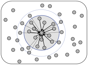
For models of distance-dependent connectivity it is necessary to assign to each model neuron a location on the two-dimensional cortical sheet. Two different algorithmic procedures can be used to assign distance-dependent connectivity (Fig. 12.11). The first one assumes full connectivity with a strength which falls off with distance
| (12.12) |
where and denote the location of post- and presynaptic neurons, respectively, and is a function into the real numbers. For convenience, one may assume finite support so that vanishes for distances .
The second alternative is to give all connections the same weight, but to assume that the probability of forming a connection depends on the distance
| (12.13) |
where and denote the location of post- and presynaptic neurons, respectively and is a function into the interval .
| A | B |
|---|---|
|
 |
Example: Expected number of connections
Let us assume that the density of cortical neurons at location is . The expected number of connection that a single neuron located at position receives is then . If the density is constant, , then the expected number of input synapses is the same for all neurons and controlled by the integral of the connection probability, i.e., .
12.3.7 Spatial Continuum Limit (*)
The physical location of a neuron in a population often reflects the task of a neuron. In the auditory system, for example, neurons are organized along an axis that reflects the neurons’ preferred frequency. A neuron at one end of the axis will respond maximally to low-frequency tones; a neuron at the other end to high frequencies. As we move along the axis the preferred frequency changes gradually. In the visual cortex, the preferred orientation changes gradually as one moves along the cortical sheet. For neurons organized in a spatially extended multidimensional network, a description by discrete pools does not seem appropriate. We will indicate in this section that a transition from discrete pools to a continuous population is possible. Here we give a short heuristic motivation of the equations. A thorough derivation along a slightly different line of arguments will be performed in Chapter 18.
To keep the notation simple, we consider a population of neurons that extends along a one-dimensional axis; cf. Fig. 12.12. We assume that the interaction between a pair of neurons depends only on their location or on the line. If the location of the presynaptic neuron is and that of the postsynaptic neuron is , then . In other words we assume full, but spatially dependent connectivity and neglect potential random components in the connectivity pattern.
In order to use the notion of population activity as defined in Eq. (12.11), we start by discretizing space in segments of size . The number of neurons in the interval is where is the spatial density. Neurons in that interval form the group .
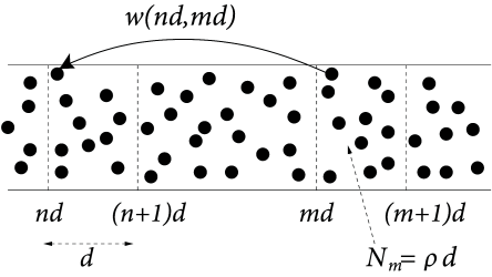
We now change our notation with respect to the discrete population and replace the subscript in the population activity by the spatial position of the neurons in that group
| (12.14) |
Since the efficacy of a pair of neurons with and is by definition with , we have . We use this in Eq. (12.11) and find for the input current
| (12.15) |
where describes the time course of the postsynaptic current caused by spike firing in one of the presynaptic neurons. For , the summation on the right-hand side can be replaced by an integral and we arrive at
| (12.16) |
which is the final result. To rephrase Eq. (12.16) in words, the input to neurons at location depends on the spatial distribution of the population activity convolved with the spatial coupling filter and the temporal filter . The population activity is the number of spikes in a short interval summed across neurons in the neighborhood around normalized by the number of neurons in that neighborhood.