Chapter 18 Cortical Field Models for Perception

The world is continuous. Humans walk along corridors and streets, move their arms, turn their head, and orient the direction of gaze. All of these movements and gestures can be described by continuous variables such as position, head direction, gaze orientation etc. These continuous variables need to be represented in the brain. Field models are designed to encode such continuous variables.

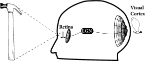
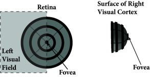
Objects such as houses, trees, cars, pencils have a finite extension in the three-dimensional space. Visual input arising from these and other objects is projected onto the retinal photoreceptors and gives rise to a two-dimensional image in the retina. This image is already preprocessed by nerve cells in the retina and undergoes some further processing stages before it arrives in cortex. A large fraction of primary visual cortex is devoted to processing of information from the retinal area around the fovea. As a consequence, the activation pattern on the cortical surface resembles a coarse, deformed and distorted image of the object (Fig. 18.1 ). Topology is largely preserved so that neighboring neurons in cortex process neighboring points of retinal space. In other words, neighboring neurons have similar receptive fields which gives rise to cortical maps; cf. Chapter 12 .

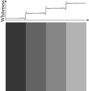
In this chapter we describe the activity of local groups of cortical neurons. We exploit the fact that neighboring neurons have similar receptive fields so as to arrive at a continuum model of cortical activity. Neural continuum models are often called field models. Neurons in a field model typically receive input on a forward path, from sensory modalities such as vision, audition, or touch, but they also interact with each other. Field models of sensory areas in cortex are suitable to explain some, but not all, aspects of perception. For example, the lateral interaction of neurons in visual cortex (and also in the retina!) gives rise to visual phenomena such as Mach-bands or grid illusions (Fig. 18.2 ).

Field models are also used for some forms of working memory. As an example, let us focus on the sense of orientation. Normally, when reading this book you are able to point spontaneously in the direction of the door of your room. Let us imagine that you spin around with closed eyes until you get dizzy and loose your sense of orientation. When you open your eyes your sense of orientation will re-establish itself based on the visual cues in your surround. Thus, visual input strongly influences self-orientation. Nevertheless, the sense of orientation also works in complete darkness. If somebody turns the lights off, you still remember where the door is. Thus, humans (and animals) have a rather stable ’internal compass’ which can be used, even in complete darkness, to walk a few steps in the right direction.

While the memory effect of the ’internal compass’ can be related to the regime of bump attractors in a continuum model, perceptual phenomena can be described by the same class of continuum models, but in the input-driven regime. Both regimes will be discussed in this chapter. We start with a general introduction to continuum models in Section 18.1 . We then turn to the input-driven regime in Section 18.2 in order to account for some perceptual and cortical phenomena. Finally we discuss the regime of bump attractors in the context of the sense of orientation (Section 18.3 ).