14.5 Adaptation in Population Equations
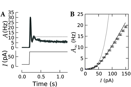
The integral equations presented so far apply only to neurons whose state does not depend on the spiking history, except on the most recent spike. Cortical neurons, however, show pronounced adaptation, as discussed in Chapter 11. Since time-dependent renewal theory cannot account for adaptation, the predicted population activity does not match the one observed in simulations; see Fig. 14.12.
As indicated in Eq. (14.12), the intuitions that have led to the integral equation (14.5) of time-dependent renewal theory, are still applicable, but the interval distribution must take into account the past history.
Let be, again, the probability of observing a spike at time given the last spike at time , the input-current and the activity history until time , then the integral equation for adapting neurons is Eq. (14.12) which we recall here for convenience
| (14.86) |
In this section, we develop the methods necessary to describe adapting neuron populations. First we present the systematic derivation of the integral equation Eq. (14.86). Then, in Section 14.5.2 we describe the event-based moment expansion which provides a framework for approximating .
14.5.1 Quasi-Renewal Theory (*)
Chapter 12 discussed the concept of a homogeneous population. We have seen that the activity of a homogeneous population of uncorrelated neurons can be seen as an average of the spike trains across the population, where the subscript denotes an average across the neurons. Because neurons are stochastic, all neurons have different spiking histories. Accordingly, an average over a population is equivalent to an average over all possible past spike trains,
| (14.87) |
where is the hazard (or instantaneous firing rate) at time given the previous spikes in the spike train and the average is over all spike train histories. In other words, can be calculated as the expected activity averaged over all possible spike train histories, whereas gives the stochastic intensity of generating a spike around time given the specific history summarized by the past spike train (358).
The spike train consists of a series of spikes , , … . To average over all possible spike trains requires that we consider spike trains made of to spikes. Moreover, for a given number of spikes, all possible time sequences of the spikes must be considered. This average takes the form of a path integral (149) where the path here is the spike trains. Therefore, the average in Eq. (14.87) is
| (14.88) |
We emphasize that in Eq. (14.88) the spikes are ordered counting backward in time; therefore is the most recent spike so that .
Each spike train can occur with a probability entirely defined by the hazard function
| (14.89) |
The equality follows from the product of two probabilities: the probabilities of observing the spikes at the times given the rest of the history (the hazard function) and the probability of not spiking between each of the spikes (the survivor function). Again, it is a generalization of the quantities seen in Chapters 7 and 9. Writing the complete path integral, we have
| (14.90) |
The case with zero spikes in the past (the first term on the right-hand-side of Eq. (14.90)) can be neglected, because we can always formally assign a firing time at to neurons that have not fired in the recent past. We now focus on the factor enclosed in square brackets on the right-hand side of Eq. (14.90). This factor resembles . In fact, if, for a moment, we made a renewal assumption, the most recent spike were the only one that mattered. This would imply that we could set inside the square brackets (where is the most recent spike) and shift the factor enclosed by square brackets in front of the integral over . In this case, the factor in square brackets would become exactly . The remaining integrals over the variables can be recognized as the average of over the possible histories, that is, . Therefore the renewal assumption leads back to Eq. (14.5), as it should.
In quasi-renewal theory, instead of assuming we assume that
| (14.91) |
where is made of all the spikes in but . This assumption is reasonable given the following two observations in real neurons. First, the strong effect of the most recent spike needs to be considered explicitly. Second, the rest of the spiking history only introduces a self-inhibition that is similar for all neurons in the population and that depends only on the expected distribution of spikes in the past (358). The approximation (14.91) is not appropriate for intrinsically bursting neurons, but should apply well to other cell types (fast-spiking, non-fast-spiking, adapting, delayed, …). If we insert Eq. (14.91) into the terms inside the square brackets of Eq. (14.90), we can define the interspike interval distribution
| (14.92) |
14.5.2 Event-based Moment Expansion (*)
The development in the previous subsection is general and does not rely on a specific neuron model nor on a specific noise model. In this section, we now introduce approximation methods that are valid for the broad class of Generalized Linear Models of spiking neurons with exponential escape noise, e.g., the Spike Response Model (see Chapter 9). The aim is to find theoretical expressions for according to quasi-renewal theory (Eq. (14.92)). In particular we need to evaluate the average of the likelihood over the past history .
We recall the SRM model with exponential escape noise (Chapter 9). The instantaneous stochastic intensity at time , given the spike history is
| (14.93) |
Here, is the input potential, describes the spike-after potential introduced by each spike and is the total membrane potential. The standard formulation of exponential escape noise, , contains two extra parameters ( for the threshold and for the noise level), but we can rescale the voltage and rate units so as to include the parameters and into the definition of and , respectively. The time course of and and the parameter can be optimized so as to describe the firing behavior of cortical neurons; cf. Chapter 11.
In the model defined by Eq. (14.93), all the history dependence is contained in a factor, , which can be factorized into the contribution from the last spike and that of all previous spikes,
| (14.94) |
In order to evaluate the expected values on the right-hand side of Eq. (14.92), we need to calculate the quantity .
is called a moment generating functional because functional derivatives with respect to and evaluated at yields the moments of : , , … . Explicit formulas for the moment generating functional are known (529). One of the expansion schemes unfolds in terms of the correlation functions and provides a useful framework for the approximation of our functional at hand.
We have already seen two examples of such correlation functions in various chapters of the book. The first term is simply the population activity , i.e., the expectation value or ‘mean’ of the spike count in a short interval . The second term in the expansion scheme, is the second-order correlation function which we have encountered in Chapter 7 in the context of autocorrelation and the noise spectrum. There, the quantity is the stationary version of the slightly more general time-dependent correlation term . Higher orders would follow the same pattern(529), but they will play no role in the following.
Using the moment expansion, the expected value in Eq. (14.94) becomes
| (14.95) |
We call the expansion the event-based moment expansion. As a physical rule of thumb, the contribution of terms in Eq. (14.95) decreases rapidly with increasing , whenever the events (i.e., spike times at times and ) are weakly coupled. For the purpose of Eq. (14.92), we can effectively ignore all second- and higher-order correlations and only keep the term with . This gives
| (14.96) |
Eq. (14.96) can be used as an excellent approximation in the survivor function as well as in formula for the interval distribution in Eq. (14.92). Used within the integral equation (14.12) it gives an implicit description of the population activity for infinite an infinite population of adapting neurons.