Chapter 15 Fast Transients and Rate Models
The mathematical formalism necessary for a correct description of the population activity in homogeneous networks of neurons is relatively involved - as we have seen Chapters 13 and 14. However, the population activity in a stationary state of asynchronous firing can simply be predicted by the neuronal gain function of isolated neurons; cf. Chapter 12. It is therefore tempting to extend the results that are valid in the stationary state to the case of time-dependent input. Let us write
| (15.1) |
where is the gain function expressed with the input potential as an argument, as opposed to input current. We choose a different symbol, because the units of the argument are different, but the relation of to the normal frequency-current curve is simply where is the single-neuron gain function for constant input at some noise level .
The input potential in the argument on the right-hand side of Eq. (15.1) is the contribution to the membrane potential that is caused by the input
| (15.2) |
where is the membrane time constant. Eq. (15.2) can also be written in the form of a differential equation
| (15.3) |
Integration of Eq. (15.3) with initial conditions in the far past leads back to Eq. (15.2) so that the two formulations are equivalent.
By construction, Eqs. (15.1) and (15.2) predict the correct population activity for a constant mean input . From Eq. (15.2) we have so that Eq. (15.1) yields the stationary activity , as it should.
The question arises whether the rate-model defined by Eqs. (15.1) and (15.2) (or, equivalently, by Eqs. (15.1) and (15.3)) is also a valid description for time-dependent stimuli. In other words, we ask whether the stationary solution of the population activity can be extended to a “quasi-stationary” rate model of the population activity. To answer this question we focus in this chapter on the special case of step stimuli. Strong step stimuli cause a transient response, which can be abrupt in networks of spiking neurons (Fig. 15.1A), but is systematically smooth and slow in the rate model defined above (Fig. 15.1B).
| A |
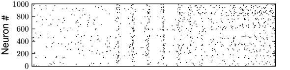
|
| B |
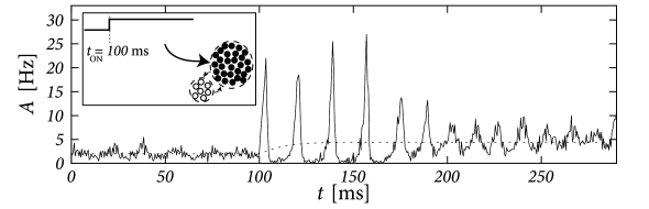 |
Therefore the question arises whether the ’normal’ case for neurons in vivo is that of an abrupt and fast response (which would be absent in the rate model), or that of a smooth and slow response as predicted by the rate model. In order to answer this question, we start in Section 15.1 by taking a closer look at experimental data.
In Section 15.2 we use modeling approaches to give an answer to the question of whether the response to a step stimulus is fast or slow. As we will see, the response of generalized integrate-and-fire models to a step input can be rapid, if the step is either strong and the noise level is low or if the noise is slow, i.e., not white. However, if the noise is white and the noise level is high, the response to the step input is slow. In this case the rate model defined above in Eqs. (15.1) and (15.2) provides an excellent approximation to the population dynamics.
Finally, in Section 15.3, we discuss several variants of rate models. We emphasize that all of the rate models discussed in this section are intended to describe the response of a population of neurons to a changing input - as opposed to rate models for single neurons. However, it is also possible to reinterpret a population model as a rate model of a single stochastically firing neuron. Indeed, the single-neuron PSTH accumulated over 200 repetitions of the same time-dependent stimulus is identical to the population activity of 200 neurons in a single trial.