15.2 Fast transients vs. slow transients in models
Populations of model neurons can exhibit fast abrupt responses or slow responses to a step current input. In order to predict whether the response is fast or slow, knowledge of the type and magnitude of noise turns out to be more critical than the details of the neuron model.
15.2.1 Fast transients for low noise or ‘slow’ noise
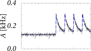
A homogeneous population of independent leaky integrate-and-fire neurons with a low level of noise exhibits a sharp transient after the onset of a step current as shown in Fig. 15.5A. The onset transiently synchronizes a subgroup of neurons. Since all the neurons are of the same type and have the same parameters, the synchronized subgroup fires again some time later, such that the population activity oscillates with a period corresponding to the inter-spike interval of single neurons.
The oscillation is suppressed and neurons desynchronize, if the population is heterogeneous or, for a homogeneous population, if neurons have slow noise in the parameters (Fig. 15.5B). The abrupt onset, however, remains so that the transient after a switch in the input is extremely fast.
| A | B |
|---|---|
|

|

|
|
We can conclude that fast transients occur in a population of leaky integrate-and-fire neurons
(i) at a low noise level and strong step-current stimulation; and
(ii) at a high level of ’slow’ noise, e.g., slow variations in the parameters of the neurons or heterogeneity across the group of neurons.
In the first case, the onset triggers oscillations, while in the second case the oscillations are suppressed. The rapid transients in spiking models without noise or with slow noise have been reported by several researchers (264; 183; 77; 351).
Note that the time course of the response in the simulations with slow noise in Fig. 15.5B is reminiscent of the neuronal responses measured in visual cortex; cf. Fig. 15.3. In particular, we find in the simulations that the rapid onset is followed by a decay of the activity immediately thereafter. This indicates that the decay of the activity is due to the reset or, more generally, to refractoriness after firing, and not due to adaptation or input from inhibitory neurons.
Whereas the low-noise result is independent of the specific noise model, the results for high noise depend on the characteristics of the noise. We analyze in the Sections 15.2.2 and 15.2.3 the response to step currents for two different noise models. We start with escape noise and turn thereafter to diffusive noise. Before we do so, let us discuss a concrete example of slow noise.
Example: Fast transients with noise in parameters
We consider a population of SRM neurons with noise in the duration of the absolute refractoriness. The membrane potential is where is the input potential and
After each spike the reset variable is chosen independently from a Gaussian distribution with variance . This is an example of a ‘slow’ noise model, because a new value of the stochastic variable is chosen only once per inter-spike interval. The approach of the neuron to the threshold is noise-free.
A neuron which was reset at time with a value fires again after an interval which is defined by the next threshold crossing . The interval distribution of the noisy reset model is
| (15.4) |
The population equation (14.5) from Chapter 14 is thus
| (15.5) |
A neuron that has been reset at time with value behaves identical to a noise-free neuron that has fired its last spike at . In particular we have the relation where is the next interspike interval of a noiseless neuron () that has fired its last spike at . The integration over in Eq. (15.5) can therefore be done and yields
| (15.6) |
where is the backward interval, i.e. the distance to the previous spike for a noiseless neuron () that fires at time . The factor arises due to the integration over the -function. We use the short-hand for the derivative and for . We remind the reader that the interval is defined by the threshold condition which gives, more explicitly, (see Exercises).
We can interpret Eq. (15.6) as follows.
(i) The activity at time is proportional to the activity one interspike interval earlier;
(ii) compared to , the activity is smoother, because interspike intervals vary across different neurons in the population which gives rise to an integration over the Gaussian ;
(iii) most importantly, compared to the activity one interspike interval earlier, the activity at time is increased by a factor . This factor is proportional to the derivative of the input potential as opposed to the potential itself. As we can see from Eq. (15.3), the derivative of is discontinuous at the moment when the step current switches. Therefore, the response of the population activity to a step current is instantaneous and exhibits an abrupt change, as confirmed by the simulation of Fig. 15.5B. We emphasize that the mathematical arguments that lead to Eq. (15.6) do neither require an assumption of small input steps nor a linearization of the population dynamics, but are applicable to arbitrary time-dependent and strong inputs.
15.2.2 Populations of neurons with escape noise
For neurons with escape noise, the level of noise determines whether transients are sharp and fast or smooth and slow. For low noise the response to a step current is fast (Fig. 15.6A) whereas for a high noise level the response is slow and follows the time course of the input potential (Fig. 15.6B). Analogous results hold for a large class of generalized integrate-and-fire models with escape noise, including SRMs and leaky integrate-and-fire models (183).
| A | B |
|---|---|

|
 |
In order to analyze the response to step current inputs, we assume that the step-amplitude of the input is small so that the population activity after the step can be considered as a small perturbation of the asynchronous firing state with activity before the step. With these assumption, we can use the linearized population activity equations (14.43) that were derived in Section 14.3 of Chapter 14. For the sake of convenience we copy the equation here
| (15.7) |
We recall that is the interval distribution for constant input before the step; is a real-valued function that plays the role of an integral kernel; and
| (15.8) |
is the input potential generated by step input of amplitude , switched on at time .
The first term on the right-hand side of Eq. (15.7) describes that perturbations in the past () have an after-effect about one inter-spike interval later. Thus, if the switch in the input at time has caused a momentary increase of the population activity , then the first peak in around can generate a second, slightly broader, peak one interspike-interval later – exactly as seen in the experimental data of Fig. 15.4A. If the second peak is again prominent, it can cause a further peak one period later, so that the population activity passes through a phase of transient oscillations; cf. Fig. 15.6A. The oscillation decays, however, rapidly if the noise level is high, because a high noise level corresponds to a broad interspike interval distribution so that successive peaks are ’smeared out’. Thus, the first term on the right-hand side of Eq. (15.7) explains the potential ’ringing’ of the population activity after a momentary synchronization of neurons around time ; it does not, however, predict whether the transient at time is sharp or not.
It is the second term on the right-hand side of Eq. (15.7) which predicts the immediate response to a change in the input potential . In the following, we are mainly interested in the initial phase of the transient, i.e. where is the mean inter-spike interval. During the initial phase of the transient, the first term on the right-hand side of Eq. (15.7) does not contribute, since for . Therefore, Eq. (15.7) reduces to
| (15.9) |
In the upper bound of the integral we have exploited that =0 for .
If we want to understand the response of the population to an input current , we need to know the characteristics of the kernel . The explicit form of the filter has been derived in Section 14.3 of Chapter 14. Here we summarize the main results that are necessary to understand the transient response of the population activity to a step current input.
-
(i)
In the low-noise limit, the kernel can be approximated by a Dirac function. The dynamics of the population activity has therefore a term proportional to the derivative of the input potential; cf. Eq. (15.9). This result implies a fast response to any change in the input. In particular, for step-current input, the response in the low-noise limit is discontinuous at the moment of the step.
-
(ii)
For a large amount of escape noise, the kernel is broad. This implies that the dynamics of the population activity is proportional to the input potential rather than to its derivative. Therefore the response to a step input is slow and consistent with that of a rate model, .
A summary of the mathematical results for the filter is given in Tab. 15.1. The formulas for leaky integrate-and-fire models differ slightly from those for SRM, because of the different treatment of the reset.
Example: Slow response for large escape noise
In order to understand how the slow response to a step at time arises, we focus on the right-hand side of Eq. (15.9) and approximate the kernel by a small constant over the interval . For (and as before , the integral simplifies then to ; i.e., a simple integral over the input potential.
In front of the integral on the right-hand side of Eq. (15.9) we see the temporal derivate. The derivate undoes the integration so that
| (15.10) |
This implies that the response to a change in the input is as slow as the input potential and controlled by the membrane time constant.
15.2.3 Populations of neurons with diffusive noise
Simulation results for a population of integrate-and-fire neurons with diffusive noise are similar to those reported for escape noise. For a small to medium amount of diffusive noise, the transient is fairly sharp and followed by a damped oscillation (Fig. 15.7A). For a large amount of noise, the oscillation is suppressed and the response of the population activity is slower (Fig. 15.7B).
In the discussion of escape noise in the preceding section, we have seen that the response to a step input is fast, if the population activity reflects the derivative of the input potential. To understand when and how the derivative can play a role with diffusive noise, it is convenient to consider for a moment not a step-current input but a current pulse. According to Eq. (15.3), a current pulse which deposits at time a charge , causes a discontinuous jump of the input potential
| (15.11) |
| A | B |
|---|---|

|
 |
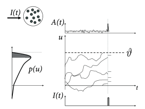
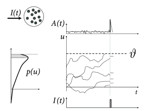
The central idea of the following arguments is shown schematically in Fig. 15.8. According to Eq. (15.11), all membrane potential trajectories jump at time by the amount . The distribution of membrane potentials across the different neurons in the population, just before , is described by . The step increase in the membrane potential kicks all neurons with membrane potential in the range instantaneously across the threshold which generates an activity pulse
| (15.12) |
where is the fraction of neurons that fire because of the input current pulse. The Dirac- pulse in the activity indicates that is proportional to the derivative of the input potential of Eq. (15.11). A population response proportional to is the signature of an immediate response to step currents.
The above argument assumes that the jump size is finite. The linearization of the membrane potential density equations (cf. Chapter 13) corresponds to the limit where the jump size goes to zero. Two different situation may occur, which are visualized in Figs. 15.8A and B, respectively. Let us start with the situation depicted in Fig. 15.8B. As the jump size goes to zero, the fraction of neurons that fire (i.e. the shaded area under the curve of ) remains proportional to . Therefore, even in the limit of to zero the linearized population equations predict a rapid response component. The fast response component is proportional , i.e., to the density of the membrane potential at threshold. For colored noise, the density at threshold is finite. Therefore, for colored noise, the response is fast (Fig. 15.9), even after linearization of the equations of the population dynamics (77; 154).
For diffusive noise with white-noise characteristics, however, the membrane potential density vanishes at the threshold. The area under the curve therefore has the shape of a triangle (Fig. 15.8A) and is proportional to . In the limit of to zero, a linearization of the equation thus predicts that the response looses its instantaneous component (78; 298; 434).
| A | B |
|---|---|
|
 |
The linearization of the membrane potential density equations leads to the linear response filter . The Fourier transform of is the frequency-dependent gain ; cf. Chapter 13. After linearization of the population activity equations, the question of fast or slow response to a step input is equivalent to the question of the high-frequency behavior of . Tab. 15.2 summarizes the main results from the literature. A cut-off frequency proportional to implies that the dynamics of the population activity is ’slow’ and roughly follows the input potential. Exponential integrate-and-fire neurons, which we have identified in Chapter 5 as a good model of cortical neurons, are always slow in this sense. If there is no cut-off, the population activity can respond rapidly. With this definition, leaky integrate-and-fire neurons respond rapidly to a change in the input variance of the diffusive noise (298; 477; 434). A cut-off proportional to means that the response of a population of leaky integrate-and-fire neurons to a step is slightly faster than that of the membrane potential but must still be considered as ’fairly slow’ (78).
We close with a conundrum: Why is the linear response of the leaky integrate-and-fire model fairly slow for all noise levels, yet the noise-free response that we have seen in Fig. 15.5A is fast? We emphasize that the linearization of the noise-free population equations does indeed predict a fast response, because, if there is no noise, the membrane potential density at the threshold is finite. However, already for a very small amount of white diffusive noise, the formal membrane potential density at the threshold vanishes, so that the linearized population equations predict a slow response. This is, however, to a certain degree an artifact of the diffusion approximation. For a small amount of diffusive noise, the layer below over which the membrane potential density drops from its maximum to zero becomes very thin. For any finite spike arrival rate and finite EPSP size in the background input or finite signal amplitude , the immediate response is strong and fast - as seen from the general arguments in Fig. 15.8.