15.3 Rate models
The gain function of rate models can always be chosen such that, for constant input , the population activity in the stationary state of asynchronous firing is correctly described. The dynamic equations that describe the approach to the stationary state in a rate model are, however, to a certain degree ad hoc. This means that the analysis of transients as well as the stability analysis in recurrent networks will, in general, give different results in rate models than in spiking neuron models.
15.3.1 Rate models have slow transients
In Section 15.2 we have seen that spiking neuron models with a large amount of escape noise exhibit a population activity that follows the input potential . In this case, it is therefore reasonable to define a rate model in which the momentary activity reflects the momentary input potential . An example is Eq. (15.1), which corresponds to a ’quasi-stationary’ treatment of the population activity, because the transform is identical to the stationary gain function, except for a change in the units of the argument, as discussed in the text after Eq. (15.1). A similar argument can also be made for exponential integrate-and-fire neurons with diffusive noise, as we will see later in this section.
If we insert Eq. (15.2) into Eq. (15.1) we find
| (15.13) |
Eq. (15.13) makes explicit that the population activity in the rate model reflects a low-pass filtered version of the input current. The transient response to a step in the input current is therefore slow.
| A | B |
|---|---|
|
 |
Since differential equations are more convenient than integrals, we rewrite the input potential in the form of Eq. (15.3) which we repeat here for convenience
| (15.14) |
The input potential resulting from the integration of Eq. (15.14) is to be inserted into the function to arrive at the population activity . Note that the input current in Eq. (15.14) can arise from external sources, from other populations or from recurrent activity in the network itself.
Example: Wilson-Cowan differential equation
Sometimes one finds in the literature rate models of the form
| (15.15) |
which have an additional time constant . Therefore the transient response to a step in the input would be even slower than that of the rate model in Eq. (15.13).
In the derivation of Wilson and Cowan (553) the time constant arises from time-averaging over the ’raw’ activity variable with a sliding window of duration . Thus, even if the ’raw’ activity has sharp transients, the time-averaged variable in Eq. (15.15) is smooth. In the theory of Wilson and Cowan, the differential equation for the population activity takes the form (552; 553)
| (15.16) |
so as to account for absolute refractoriness of duration ; cf. the integral equation (14.10) in Chapter 14. has a sigmoidal shape. The input potential comprises input from the same as well as from other populations.
Since there is no reason to introduce the additional low-pass filter with time constant , we advise against the use of the model defined in Eqs. (15.15) or (15.16). However, we may set
| (15.17) |
where is the input current (as opposed to the input potential). The current can be attributed to input from other populations or from recurrent coupling within the population. The low-pass filter in Eq. (15.17) replaces the low-pass filter in Eq. (15.14) so that the two rate models are equivalent after an appropriate rescaling of the input, even for complex networks (345); see also Exercises.
15.3.2 Networks of rate models
Let us consider a network consisting of populations. Each population contains a homogeneous population of neurons. The input into population arising from other populations and from recurrent coupling within the population is described as
| (15.18) |
Here is the activity of population and is the number of presynaptic neurons in population that are connected to a typical neuron in population ; the time course and strength of synaptic connections are described by and , respectively; see Chapter 12.
We describe the dynamics of the input potential of population with the differential equation (15.14) and use for each population the quasi-stationary rate model where is the gain function of the neurons in population . The final result is
| (15.19) |
Eq. (15.19) is the starting point for some of the models in Part IV of this book.
Example: Population with self-coupling
If we have a single population, we can drop the indices in Eq. (15.19) so as to arrive at
| (15.20) |
where is the strength of the feedback. Thus, a single population with self-coupling is described by a single differential equation for the input potential . The population activity is simply .
Stationary states are found as discussed in Chapter 12. If there are three fixed points, the middle one is unstable while the other two (at low and high activity, respectively) are stable under the dynamics (15.20). The fixed points calculated from Eq. (15.20) are correct. However, stability under the dynamics (15.20) does not guarantee stability of the original network of spiking neurons. Indeed, as we have seen in Chapters 13 and 14, the fixed points of high and low activity may loose stability with respect to oscillations, even in a single homogeneous population. The rate dynamics of Eq. (15.20) cannot correctly account for these oscillations. In fact, for instantaneous synaptic current pulses , where denotes the Dirac -function, Eq. (15.20) reduces to a one-dimensional differential equation which can never give rise to oscillatory solutions.
15.3.3 Linear-Nonlinear-Poisson and improved transients
To improve the description of transients, we start from Eq. (15.13), but insert an arbitrary filter ,
| (15.21) |
Eq. (15.21) is called the Linear-Nonlinear-Poisson (LNP) model (94; 478). It is also called a cascade model because it can be interpreted as a sequence of three processing steps. First, input is filtered with an arbitrary linear filter , which yields the input potential . Second, the result is passed through a nonlinearity . Third, in case of a single neurons, spikes are generated by an inhomogeneous Poisson process with rate . Since, in our model of a homogeneous population, we have many similar neurons, we drop the third step and interpret the rate directly as the population activity.
For we are back at Eq. (15.13). The question arises whether we can make a better choice of the filter than a simple low-pass with the membrane time constant . In Chapter 11 it is shown how an optimal filter can be determined experimentally by reverse correlation techniques.
Here we are interested in deriving the optimal filter from the complete population dynamics. The LNP model in Eq. (15.21) is an approximation of the population dynamics that is more correctly described by the Fokker-Planck equations in Ch. 13 or by the integral equation of time-dependent renewal theory in Ch. 14. Let us recall that in both approaches, we can linearize the population equations around a stationary state of asynchronous firing which is obtained with a mean input at some noise level . The linearization of the population dynamics about yields a filter . We use this filter, and arrive at a variant of Eq. (15.21)
| (15.22) |
where is a scaled version of the frequency-current curve and a constant which matches the slope of the gain function at the reference point for the linearization (373). Models with this, or similar choices of , describe transient peaks in the population activity surprisingly well; see e.g., (214; 33; 373).
Rate models based on Eq. (15.22) can also be used to describe coupled populations. Stability of a stationary state is correctly described by Eq. (15.22), if the filter in the argument on the right-hand-side reflects the linearization of the full population dynamics around , but not if the filter is derived by linearization around some other value of the activity.
Example: Effective rate model for Exponential Integrate-and-Fire neurons
We denote the stationary gain function of exponential integrate-and-fire neurons by and the linear filter arising from linearization around a stationary activity by . For exponential integrate-and-fire neurons has the high-frequency behavior of a low-pass filter ; see Tab. 15.2.
We recall that the Fourier-transform of an exponential filter also yields a high-frequency behavior with the inverse filter time constant as cut-off frequency. This suggests that, for the exponential integrate-and-fire model, we can approximate the time course of as an exponential filter with an effective time constant . This leads back to Eq. (15.22), but with an exponential filter . Hence, we are now nearly back to Eq. (15.13), except that the time constant of the exponential is different.
We now switch from the frequency current curve to the equivalent description of the gain function where the argument of has units of a potential. It is convenient to implement the exponential filter in the form of a differential equation for the the input potential (373)
| (15.23) |
with an effective time constant
| (15.24) |
where is the activity averaged over one or a few previous time steps and is the derivative of the gain function at an appropriately chosen reference point , so that is the long-term average of the activity.
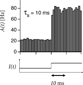
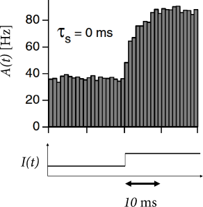
In each time step, we update the input using Eq. (15.23) and calculate the activity as with . Such a rate model gives an excellent approximation of the activity in a population of exponential integrate-and-fire neurons (Fig. 15.10). Note that fast transients are well described, because the effective time constant is shortened as soon as the population activity increases.
 |
 |
15.3.4 Adaptation
So far we have focused on the initial transient after a step in the input current. After the initial transient, however, follows a second, much slower phase of adaptation during which the population response decreases, even if the stimulation is kept constant. For single neurons, adaptation has been discussed in Chapter 6.
In a population of neurons, adaptation can be described as an effective decrease in the input potential. If a population of non-adaptive neurons has an activity described by the gain function , then the population rate model for adaptive neurons is
| (15.25) |
where describes the amount of adaptation that neurons have accumulated
| (15.26) |
where is the asymptotic level of adaptation that is attained if the population continuously fires at a constant rate . The asymptotic level is approached with a time constant . Eqs. (15.25) and (15.26) are a simplified version of the phenomenological model proposed in Benda and Herz (48).
Example: Effective adaptation filter
Suppose that is linear in the population activity with a constant and is independent of . Then Eq. (15.26) can be integrated and yields with a filter . We insert the result in Eq. (15.25) and find
| (15.27) |
Eq. (15.27) nicely describes the adaptation process but it misses, like other rate models, the sharp initial transient, and potential transient oscillation, caused by the synchronization of the population at the moment of the step (358)