19 Synaptic Plasticity and Learning 19.1 Hebb rule and experiments 19.3 Unsupervised learning

19.2 Models of Hebbian learning

Before we turn to spike-based learning rules, we first review the basic concepts of correlation-based learning in a firing rate formalism. Firing rate models (cf. Ch. 15 ) have been used extensively in the field of artificial neural networks; cf. Hertz et al. ( 215 ) ; Haykin ( 209 ) for reviews.

19.2.1 A Mathematical Formulation of Hebb’s Rule

In order to find a mathematically formulated learning rule based on Hebb’s postulate we focus on a single synapse with efficacy $w_{ij}$ that transmits signals from a presynaptic neuron $j$ to a postsynaptic neuron $i$ . For the time being we content ourselves with a description in terms of mean firing rates. In the following, the activity of the presynaptic neuron is denoted by $\nu_{j}$ and that of the postsynaptic neuron by $\nu_{i}$ .

There are two aspects in Hebb’s postulate that are particularly important; these are locality and joint activity . Locality means that the change of the synaptic efficacy can only depend on local variables, i.e., on information that is available at the site of the synapse, such as pre- and postsynaptic firing rate, and the actual value of the synaptic efficacy, but not on the activity of other neurons. Based on the locality of Hebbian plasticity we can write down a rather general formula for the change of the synaptic efficacy,

{{\text{d}}\over{\text{d}}t}w_{ij}=F(w_{ij};\nu_{i},\nu_{j})\,.

(19.1)

Here, ${{\text{d}}w_{ij}/{\text{d}}t}$ is the rate of change of the synaptic coupling strength and $F$ is a so far undetermined function ( 465 ) . We may wonder whether there are other local variables (e.g., the input potential $h_{i}$ , cf. Ch. 15 ) that should be included as additional arguments of the function $F$ . It turns out that in standard rate models this is not necessary, since the input potential $h_{i}$ is uniquely determined by the postsynaptic firing rate, $\nu_{i}=g(h_{i})$ , with a monotone gain function $g$ .

The second important aspect of Hebb’s postulate is the notion of ‘joint activity’ which implies that pre- and postsynaptic neurons have to be active simultaneously for a synaptic weight change to occur. We can use this property to learn something about the function $F$ . If $F$ is sufficiently well-behaved, we can expand $F$ in a Taylor series about $\nu_{i}=\nu_{j}=0$ ,

	$\displaystyle{{\text{d}}\over{\text{d}}t}w_{ij}$	$\displaystyle=c_{0}(w_{ij})+c^{\text{pre}}_{1}(w_{ij})\,\nu_{j}+c^{\text{post}% }_{1}(w_{ij})\nu_{i}+c^{\text{pre}}_{2}(w_{ij})\,\nu_{j}^{2}$
		$\displaystyle\qquad+c^{\text{post}}_{2}(w_{ij})\,\nu_{i}^{2}+c^{\text{corr}}_{% 11}(w_{ij})\,\nu_{i}\,\nu_{j}+{\mathcal{O}}(\nu^{3})\,.$		(19.2)

The term containing $c^{\text{corr}}_{11}$ on the right-hand side of ( 19.2.1 ) is bilinear in pre- and postsynaptic activity. This term implements the AND condition for joint activity. If the Taylor expansion had been stopped before the bilinear term, the learning rule would be called ‘non-Hebbian’, because pre- or postsynaptic activity alone induces a change of the synaptic efficacy and joint activity is irrelevant. Thus a Hebbian learning rule needs either the bilinear term $c^{\text{corr}}_{11}(w_{ij})\,\nu_{i}\,\nu_{j}$ with $c^{\text{corr}}_{11}>0$ or a higher-order term (such as $c_{21}(w_{ij})\,\nu_{i}^{2}\,\nu_{j}$ ) that involves the activity of both pre- and postsynaptic neurons.

Example: Hebb rules, saturation, and LTD

The simplest choice for a Hebbian learning rule within the Taylor expansion of Eq. ( 19.2.1 ) is to fix $c^{\text{corr}}_{11}$ at a positive constant and to set all other terms in the Taylor expansion to zero. The result is the prototype of Hebbian learning,

{{\text{d}}\over{\text{d}}t}w_{ij}=c^{\text{corr}}_{11}\,\nu_{i}\,\nu_{j}\,.

(19.3)

We note in passing that a learning rule with $c^{\text{corr}}_{11}<0$ is usually called anti-Hebbian because it weakens the synapse if pre- and postsynaptic neuron are active simultaneously; a behavior that is just contrary to that postulated by Hebb.

Note that, in general, the coefficient $c^{\text{corr}}_{11}$ may depend on the current value of the weight $w_{ij}$ . This dependence can be used to limit the growth of weights at a maximum value $w^{\rm max}$ . The two standard choices of weight-dependence are called ’hard bound’ and ‘soft bound’, respectively. Hard bound means that $c^{\text{corr}}_{11}=\gamma_{2}$ is constant in the range $0<w_{ij}<w^{\rm max}$ and zero otherwise. Thus, weight growth stops abruptly if $w_{ij}$ reaches the upper bound $w^{\rm max}$ .

A soft bound for the growth of synaptic weights can be achieved if the parameter $c^{\text{corr}}_{11}$ in Eq. ( 19.3 ) tends to zero as $w_{ij}$ approaches its maximum value $w^{\rm max}$ ,

c^{\text{corr}}_{11}(w_{ij})=\gamma_{2}\,(w^{\rm max}-w_{ij})^{\beta}\,,

(19.4)

with positive constants $\gamma_{2}$ and $\beta$ . The typical value of the exponent is $\beta=1$ , but other choices are equally possible ( 202 ) . For $\beta\to 0$ , the soft-bound rule ( 19.4 ) converges to the hard-bound one.

Note that neither Hebb’s original proposal nor the simple rule ( 19.3 ) contain a possibility for a decrease of synaptic weights. However, in a system where synapses can only be strengthened, all efficacies will eventually saturate at their upper maximum value. Our formulation ( 19.2.1 ) is sufficiently general to allow for a combination of synaptic potentiation and depression. For example, if we set $w^{\rm max}=\beta=1$ in ( 19.4 ) and combine it with a choice $c_{0}(w_{ij})=-\gamma_{0}\,w_{ij}$ , we obtain a learning rule

{{\text{d}}\over{\text{d}}t}w_{ij}=\gamma_{2}\,(1-w_{ij})\,\nu_{i}\,\nu_{j}-% \gamma_{0}\,w_{ij}\,,

(19.5)

where, in the absence of stimulation, synapses spontaneously decay back to zero. Many other combinations of the parameters $c_{0}\dots c^{\text{corr}}_{11}$ in Eq. ( 19.2.1 ) exist. They all give rise to valid Hebbian learning rules that exhibit both potentiation and depression; cf. Table 19.1 .

${\rm post}$	${\rm pre}$	${{\text{d}}w_{ij}/{\text{d}}t}\propto$	${{\text{d}}w_{ij}/{\text{d}}t}\propto$	${{\text{d}}w_{ij}/{\text{d}}t}\propto$	${{\text{d}}w_{ij}/{\text{d}}t}\propto$	${{\text{d}}w_{ij}/{\text{d}}t}\propto$
$\nu_{i}$	$\nu_{j}$	${\nu_{i}\,\nu_{j}}$	${\nu_{i}\,\nu_{j}-c_{0}}$	${(\nu_{i}\!-\!\nu_{\theta})\,\nu_{j}}$	${\nu_{i}\,(\nu_{j}\!-\!\nu_{\theta})}$	${(\nu_{i}\!-\!\langle\nu_{i}\rangle)(\nu_{j}\!-\!\langle\nu_{j}\rangle)}$
ON	ON	+	+	+	+	+
ON	OFF	0	$-$	0	$-$	$-$
OFF	ON	0	$-$	$-$	0	$-$
OFF	OFF	0	$-$	0	0	+

Table 19.1: The change

{{\text{d}}\over{\text{d}}t}w_{ij}

of a synapse from

j

i

for various Hebb rules as a function of pre- and postsynaptic activity. ‘ON’ indicates a neuron firing at high rate (

\nu>0

), whereas ‘OFF’ means an inactive neuron (

\nu=0

). From left to right: Standard Hebb rule, Hebb with decay, Hebb with postsynaptic or presynaptic LTP/LTD threshold, covariance rule. The parameters are

0<\nu_{\theta}<\nu^{\rm max}

and

0<c_{0}<(\nu^{\rm max})^{2}

Example: Covariance rule

Sejnowski ( 467 ) has suggested a learning rule of the form

{{\rm d}\over{\rm{\text{d}}t}}w_{ij}=\gamma\,\left(\nu_{i}-\langle\nu_{i}% \rangle\right)\,\left(\nu_{j}-\langle\nu_{j}\rangle\right)\,,

(19.6)

called covariance rule. This rule is based on the idea that the rates $\nu_{i}(t)$ and $\nu_{j}(t)$ fluctuate around mean values $\langle\nu_{i}\rangle,\langle\nu_{j}\rangle$ that are taken as running averages over the recent firing history. To allow a mapping of the covariance rule to the general framework of Eq. ( 19.2.1 ), the mean firing rates $\langle\nu_{i}\rangle$ and $\langle\nu_{j}\rangle$ have to be constant in time.

Example: Oja’s rule

All of the above learning rules had $c^{\text{pre}}_{2}=c^{\text{post}}_{2}=0$ . Let us now consider a nonzero quadratic term $c^{\text{post}}_{2}=-\gamma\,w_{ij}$ . We take $c^{\text{corr}}_{11}=\gamma>0$ and set all other parameters to zero. The learning rule

{{\text{d}}\over{\text{d}}t}w_{ij}=\gamma\,[\nu_{i}\,\nu_{j}-w_{ij}\,\nu_{i}^{% 2}]

(19.7)

is called Oja’s rule ( 369 ) . Under some general conditions Oja’s rule converges asymptotically to synaptic weights that are normalized to $\sum_{j}w_{ij}^{2}=1$ while keeping the essential Hebbian properties of the standard rule of Eq. ( 19.3 ); see Exercises. We note that normalization of $\sum_{j}w_{ij}^{2}$ implies competition between the synapses that make connections to the same postsynaptic neuron, i.e., if some weights grow, others must decrease.

Example: Bienenstock-Cooper-Munro rule

Higher-order terms in the expansion on the right-hand side of Eq. ( 19.2.1 ) lead to more intricate plasticity schemes. Let us consider

{{\text{d}}\over{\text{d}}t}w_{ij}=\phi\,(\nu_{i}-\nu_{\theta})\,\nu_{j}\,

(19.8)

with a nonlinear function $\phi$ and a reference rate $\nu_{\theta}$ . If we take $\nu_{\theta}$ to be a function $f(\langle\nu_{i}\rangle)$ of the average output rate $\langle\nu_{i}\rangle$ , then we obtain the so-called Bienenstock-Cooper-Munro (BCM) rule ( 58 ) .

The basic structure of the function $\phi$ is sketched in Fig. 19.5 . If presynaptic activity is combined with moderate levels of postsynaptic excitation, the efficacy of synapses activated by presynaptic input is decreased . Weights are increased only if the level of postsynaptic activity exceeds a threshold, $\nu_{\theta}$ . The change of weights is restricted to those synapses which are activated by presynaptic input. A common choice for the function $\phi$ is

{{\text{d}}\over{\text{d}}t}w_{ij}=\eta\,\nu_{i}\,(\nu_{i}-\nu_{\theta})\,\nu_% {j}=c_{21}\nu_{i}^{2}\nu_{j}-c^{\text{corr}}_{11}\nu_{i}\nu_{j}

(19.9)

which can be mapped to the Taylor expansion of Eq. ( 19.2.1 ) with $c_{21}=\eta$ and $c^{\text{corr}}_{11}=-\eta\nu_{\theta}$ .

For stationary input, it can be shown that the postsynaptic rate $\nu_{i}$ under the BCM-rule ( 19.9 ) has a fixed point at $\nu_{\theta}$ which is unstable (see Exercises). In order to avoid that the postsynaptic firing rate blows up or decays to zero, it is therefore necessary to turn $\nu_{\theta}$ into an adaptive variable which depends on the average rate $\langle\nu_{i}\rangle$ . The BCM rule leads to input selectivity (see Exercises) and has been successfully used to describe the development of receptive fields ( 58 ) .

Fig. 19.5: BCM rule. Synaptic plasticity is characterized by two thresholds for the postsynaptic activity (58). Below $\nu_{0}$ no synaptic modification occurs, between $\nu_{0}$ and $\nu_{\theta}$ synapses are depressed, and for postsynaptic firing rates beyond $\nu_{\theta}$ synaptic potentiation can be observed. Often $\nu_{0}$ is set to zero.

19.2.2 Pair-based Models of STDP

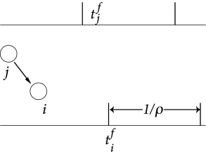
We now switch from rate-based models of synaptic plasticity to a description with spikes. Suppose a presynaptic spike occurs at time $t_{\mathrm{pre}}$ and a postsynaptic one at time $t_{\mathrm{post}}$ . Most models of STDP interpret the biological evidence in terms of a pair-based update rule, i.e. the change in weight of a synapse depends on the temporal difference $|\Delta t|=|t_{\mathrm{post}}-t_{\mathrm{pre}}|$ ; cf. Fig. 19.4 F. In the simplest model, the updates are

	$\displaystyle\Delta w_{+}$	$\displaystyle=$	$\displaystyle A_{+}(w)\cdot\exp(-\left\|\Delta t\right\|/\tau_{+})\mbox{ at }t_{% \mathrm{post}}\quad\mbox{for}\;t_{\mathrm{pre}}<t_{\mathrm{post}}$
	$\displaystyle\Delta w_{-}$	$\displaystyle=$	$\displaystyle A_{-}(w)\cdot\exp(-\left\|\Delta t\right\|/\tau_{-})\mbox{ at }t_{% \mathrm{pre}}\quad\mbox{for}\;t_{\mathrm{pre}}>t_{\mathrm{post}}$		(19.10)

where $A_{\pm}(w)$ describes the dependence of the update on the current weight of the synapse. Usually $A_{\pm}(w)$ is positive and $A_{\pm}(w)$ is negative. The update of synaptic weights happens immediately after each presynaptic spike (at time $t_{\rm pre}$ ) and each postsynaptic spike (at time $t_{\rm post}$ ). A pair-based model is fully specified by defining: (i) the weight-dependence of the amplitude parameter $A_{\pm}(w)$ ; (ii) which pairs are taken into consideration to perform an update. A simple choice is to take all pairs into account. An alternative is to consider for each postsynaptic spike only the nearest presynaptic spike or vice versa. Note that spikes that are far apart hardly contribute because of the exponentially fast decay of the update amplitude with the interval $|\Delta t|$ . Instead of an exponential decay ( 489 ) , some other arbitrary time-dependence, described by a learning window $W_{+}(s)$ for LTP and $W_{-}(s)$ for LTD is also possible ( 176; 256 ) .

If we introduce $S_{j}=\sum_{f}\delta(t-t_{j}^{(f)})$ and $S_{i}=\sum_{f}\delta(t-t_{i}^{(f)})$ for the spike trains of pre- and postsynaptic neurons, respectively, then we can write the update rule in the form ( 262 )

	$\displaystyle\frac{{\text{d}}}{{\text{d}}t}w_{ij}(t)=$	$\displaystyle S_{j}(t)\,\left[a_{1}^{\text{pre}}+\int_{0}^{\infty}A_{-}(w_{ij}% )W_{-}(s)\,S_{i}(t-s)\;{\text{d}}s\right]$
		$\displaystyle+S_{i}(t)\,\left[a_{1}^{\text{post}}+\int_{0}^{\infty}A_{+}(w_{ij% })W_{+}(s)\,S_{j}(t-s)\;{\text{d}}s\right]\,,$		(19.11)

where $W_{\pm}$ denotes the time course of the learning window while $a_{1}^{\text{pre}}$ and $a_{1}^{\text{post}}$ are non-Hebbian contributions, analogous to the parameters $c^{\text{pre}}_{1}$ and $c^{\text{post}}_{1}$ in the rate-based model of Eq. 19.2.1 . In the standard pair-based STDP rule, we have $W_{\pm}(s)=\exp(-s/\tau_{\pm})$ and $a_{1}^{\text{pre}}=a_{1}^{\text{post}}=0$ ; cf. Eq. ( 19.10 ).

Example: Implementation by local variables

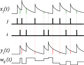
The pair-based STDP rule of Eq. ( 19.10 ) can be implemented with two local variables, i.e. one for a low-pass filtered version of the presynaptic spike train and one for the postsynaptic spikes. Suppose that each presynaptic spike at synapse $j$ leaves a trace $x_{j}$ , i.e. its update rule is

{{\text{d}}x_{j}\over{\text{d}}t}=-{x_{j}\over\tau_{+}}+\sum_{f}\delta(t-t_{j}% ^{f})

(19.12)

where $t_{j}^{f}$ if the firing time of the presynaptic neuron. In other words, the variable is increased by an amount of one at the moment of a presynaptic spike and decreases exponentially with time constant $\tau_{+}$ afterward. Similarly, each postsynaptic spike leaves a trace $y_{i}$

{{\text{d}}y_{i}\over{\text{d}}t}=-{y_{i}\over\tau_{-}}+\sum_{f}\delta(t-t_{i}% ^{f})\,.

(19.13)

The traces $x_{j}$ and $y_{i}$ play an important role during the weight update. At the moment of a presynaptic spike, a decrease of the weight is induced proportional to the value of the postsynaptic trace $y_{i}$ . Analogously, potentiation of the weight occurs at the moment of a postsynaptic spike proportional to the trace $x_{j}$ left by a previous presynaptic spike,

{\text{d}}w_{ij}/{\text{d}}t=A_{-}(w_{ij})y_{i}(t)\sum_{f}\delta(t-t_{j}^{f})% +A_{+}(w_{ij})x_{j}(t)\sum_{f}\delta(t-t_{i}^{f})\,.

(19.14)

The traces $x_{j}$ and $y_{i}$ correspond here to the factors $\exp(-|\Delta t|/\tau_{\pm})$ in Eq. ( 19.10 ). For the weight-dependence of the factors $A_{-}$ and $A_{+}$ , one can use either hard bounds or soft bounds; cf. Eq. ( 19.4 ).

Fig. 19.6: Implementation of pair-based plasticity by local variables: The presynaptic spikes leave a trace $x_{j}(t)$ , postsynaptic spikes a trace $y_{i}(t)$ . The weight increases at the moment of a postsynaptic spike proportional to the momentary value of the trace $x_{j}(t)$ left by previous presynaptic spike arrivals. Analogously we get depression for post-before-pre pairings at the moment of a presynaptic spike (vertical dashed lines highlight moments of spike firing); from Morrison et al. (353).

19.2.3 Generalized STDP models

There is considerable evidence that the pair-based STDP rule discussed above cannot give a full account of experimental results with STDP protocols. Specifically, they reproduce neither the dependence of plasticity on the repetition frequency of pairs of spikes in an experimental protocol, nor the results of triplet and quadruplet experiments.

STDP experiments are usually carried out with about $50-60$ pairs of spikes. The temporal distance of the spikes in the pair is of the order of a few to tens of milliseconds, whereas the temporal distance between the pairs is of the order of hundreds of milliseconds to seconds. In the case of a potentiation protocol (i.e. pre-before-post), standard pair-based STDP models predict that if the repetition frequency $\rho$ is increased, the strength of the depressing interaction (i.e. post-before-pre) becomes greater, leading to less net potentiation. However, experiments show that increasing the repetition frequency leads to an increase in potentiation ( 483; 468 ) . Other experimentalists have employed multiple-spike protocols, such as repeated presentations of symmetric triplets of the form pre-post-pre and post-pre-post ( 53; 160; 542; 159 ) . Standard pair-based models predict that the two sequences should give the same results, as they each contain one pre-post pair and one post-pre pair. Experimentally, this is not the case.

Here we review two examples of simple models which account for these experimental findings ( 394; 99 ) , but there are other models which also reproduce frequency dependence, e.g., ( 469 ) .

Triplet model

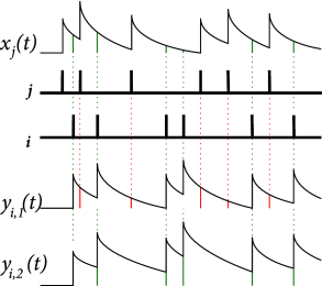
Fig. 19.7: Implementation of the triplet rule by local variables. The spikes of a presynaptic neuron $j$ contribute to a trace $x_{j}(t)$ , the spikes of postsynaptic neuron $i$ contribute to a fast trace $y_{i,1}(t)$ and a slow trace $y_{i,2}(t)$ . The update of the weight $w_{ij}$ at the moment of a presynaptic spike is proportional to the momentary value of the fast trace $y_{i,1}(t)$ , as in the pair-based model of Fig. 19.6. The update of the weight $w_{ij}$ at the moment of a postsynaptic spike is proportional to the momentary value of the trace $x_{j}(t)$ and the value of the slow trace $y_{i,2}(t)$ just before the spike. Moments of weight update are indicated by vertical dashed lines; from Morrison et al. (353)

One simple approach to modeling STDP which addresses the issues of frequency dependence is the triplet rule developed by Pfister and Gerstner ( 394 ) . In this model, LTP is based on sets of three spikes (one presynaptic and two postsynaptic). The triplet rule can be implemented with local variables as follows. Similarly to pair-based rules, each spike from presynaptic neuron $j$ contributes to a trace $x_{j}$ at the synapse:

\displaystyle\frac{{\text{d}}x_{j}}{{\text{d}}t}

\displaystyle=-

\displaystyle\frac{x_{j}}{\tau_{+}}+\sum_{t_{j}^{f}}\delta\left(t-t_{j}^{f}% \right)\,,

where $t_{j}^{f}$ denotes the firing times of the presynaptic neuron. Unlike pair-based rules, each spike from postsynaptic neuron $i$ contributes to a fast trace $y_{i,1}$ and a slow trace $y_{i,2}$ at the synapse:

	$\displaystyle\frac{{\text{d}}y_{i,1}}{{\text{d}}t}$	$\displaystyle=$	$\displaystyle-\frac{y_{i,1}}{\tau_{1}}+\sum_{f}\delta(t-t_{i}^{f})$
	$\displaystyle\frac{{\text{d}}y_{i,2}}{{\text{d}}t}$	$\displaystyle=$	$\displaystyle-\frac{y_{i,2}}{\tau_{2}}+\sum_{f}\delta(t-t_{i}^{f})\>,$

where $\tau_{1}<\tau_{2}$ , see Fig. 19.7 . The new feature of the rule is that LTP is induced by a triplet effect: the weight change is proportional to the value of the presynaptic trace $x_{j}$ evaluated at the moment of a postsynaptic spike and also to the slow postsynaptic trace $y_{i,2}$ remaining from previous postsynaptic spikes:

\Delta w_{ij}^{+}\left(t_{i}^{f}\right)=A_{+}\left(w_{ij}\right)\,x_{j}\left(t% _{i}^{f}\right)y_{i,2}\left(t_{i}^{f-}\right)

(19.15)

where $t_{i}^{f-}$ indicates that the function $y_{i,2}$ is to be evaluated before it is incremented due to the postsynaptic spike at $t_{i}^{f}$ . LTD is analogous to the pair-based rule, given in 19.14 , i.e. the weight change is proportional to the value of the fast postsynaptic trace $y_{i,1}$ evaluated at the moment of a presynaptic spike.

Fig. 19.8: Frequency dependence of STDP. A The experimental protocol depicted in Fig. 19.4 was repeated for different frequency, $\rho$ of pre-post pairs. B. The triplet rule reproduces the finding that increased frequency of pair repetition leads to increased potentiation in visual cortex pyramidal neurons. Top curve $t^{(f)}_{i}-t^{(f)}_{j}=10$ ms, bottom curve -10 ms. Data from Sjöström et al. (483), figure adapted from Pfister et al. (396).

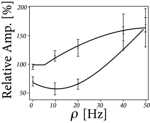
The triplet rule reproduces experimental data from visual cortical slices ( 483 ) that increasing the repetition frequency in the STDP pairing protocol increases net potentiation ( 19.8 ). It also gives a good fit to experiments based on triplet protocols in hippocampal culture ( 542 ) .

The main functional advantage of such a triplet learning rule is that it can be mapped to the BCM rule of Eqs. ( 19.8 ) and ( 19.9 ): if we assume that the pre- and postsynaptic spike trains are governed by Poisson statistics, the triplet rule exhibits depression for low postsynaptic firing rates and potentiation for high postsynaptic firing rates ( 394 ) ; see Exercises. If we further assume that the triplet term in the learning rule depends on the mean postsynaptic frequency, a sliding threshold between potentiation and depression can be defined. In this way, the learning rule matches the requirements of the BCM theory and inherits the properties of the BCM learning rule such as the input selectivity (see exercises). From the BCM properties, we can immediately conclude that the triplet model should be useful for receptive field development ( 58 ) .

Example: Plasticity model with voltage dependence

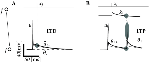
Spike timing dependence is only one of several manifestations of synaptic plasticity. Apart from spike timing, synaptic plasticity also depends on several other variables, in particular on postsynaptic voltage (Fig. 19.3 ). In this example, we present the voltage-dependent model of ( 99 ) .

The Clopath model exhibits separate additive contributions to the plasticity rule, one for LTD and another one for LTP. For the LTD part, presynaptic spike arrival at a synapse from a presynaptic neuron $j$ to a postsynaptic neuron $i$ induces depression of the synaptic weight $w_{ij}$ by an amount $-A_{\rm LTD}\,[\overline{u}_{i,-}(t)-\theta_{-}]_{+}$ that is proportional to the average postsynaptic depolarization $\overline{u}_{i,-}$ . The brackets $[\,]_{+}$ indicate rectification, i.e. any value $\overline{u}_{i,-}<\theta_{-}$ does not lead to a change; cf. Artola et al. ( 29 ) and Fig. 19.3 . The quantity $\overline{u}_{i,-}(t)$ is an low-pass filtered version of the postsynaptic membrane potential $u(t)$ with a time constant $\tau_{-}$ :

\tau_{-}\frac{{\text{d}}}{{\text{d}}t}\overline{u}_{i,-}(t)=-\overline{u}_{i,-% }(t)+u_{i}(t).

Introducing the presynaptic spike train $S_{j}(t)=\sum_{f}\delta(t-t^{f}_{j})$ , the update rule for depression is (Fig. 19.9 )

\displaystyle\frac{{\text{d}}}{{\text{d}}t}w^{\rm LTD}_{ij}=-A_{\rm LTD}(\bar{% u_{i}})\>S_{j}(t)\>[\overline{u}_{i,-}(t)-\theta_{-}]_{+}\qquad\rm\rm{if}\it\;% w_{ij}>w_{\rm min},

(19.16)

where $A_{\rm LTD}(\bar{u}_{i})$ is an amplitude parameter that depends on the mean depolarization $\bar{u}$ of the postsynaptic neuron, averaged over a time scale of 1 second. A choice $A_{\rm LTD}(\bar{u}_{i})=\alpha\,\frac{\bar{u}_{i}^{2}}{u_{ref}^{2}}$ where $u^{2}_{ref}$ is a reference value, is a simple method to avoid a run-away of the rate of the postsynaptic neuron, analogous to the sliding threshold in the BCM rule of Eq. ( 19.9 ). A comparison with the triplet rule above shows that the role of the trace $y_{i}$ (which represents a low-pass filter of the postsynaptic spike train, cf. Eq. ( 19.13 )) is taken over by the low-pass filter $\overline{u}_{i,-}$ of the postsynaptic voltage.

For the LTP part, we assume that each presynaptic spike at the synapse $w_{ij}$ increases the trace $\bar{x}_{j}(t)$ of some biophysical quantity, which decays exponentially with a time constant $\tau_{+}$ in the absence of presynaptic spikes; cf. Eq. ( 19.12 ). The potentiation of $w_{ij}$ depends on the trace $\bar{x}_{j}(t)$ and the postsynaptic voltage via (see also Fig. 19.9 )

\displaystyle\frac{{\text{d}}}{{\text{d}}t}w^{\rm LTP}_{ij}=+A_{\rm LTP}\>\bar{% x}_{j}(t)\>[u_{i}(t)-\theta_{+}]_{+}\>[\overline{u}_{i,+}(t)-\theta_{-}]_{+}% \qquad\rm{if}\it\;w_{ij}<w_{\rm max}.

(19.17)

Here, $A_{\rm LTP}>0$ is a constant parameter and $\overline{u}_{i,+}(t)$ is another low-pass filtered version of $u_{i}(t)$ similar to $\overline{u}_{-}(t)$ but with a shorter time constant $\tau_{+}$ around 10ms. Thus positive weight changes can occur if the momentary voltage $u_{i}(t)$ surpasses a threshold $\theta_{+}$ and, at the same time the average value $\overline{u}_{i,+}(t)$ is above $\theta_{-}$ . Note again the similarity to the triplet STDP rule. If the postsynaptic voltage is dominated by spikes, so that $u_{i}(t)=\sum_{f}\delta(t-t_{i}^{(f)})$ the Clopath model and the triple STDP rule are in fact equivalent.

The Clopath rule is summarized by the equation

\displaystyle\frac{{\text{d}}}{{\text{d}}t}w_{ij}=-A_{\rm LTD}(\bar{u}_{i})\,S_{j}% (t)\,[\overline{u}_{i,-}(t)-\theta_{-}]_{+}+A_{\rm LTP}\,\bar{x}_{j}(t)\,[u_{i% }(t)-\theta_{+}]_{+}\,[\overline{u}_{i,+}(t)-\theta_{-}]_{+},

(19.18)

combined with hard bounds $0\leq w_{ij}\leq w_{max}$ .

The plasticity rule can be fitted to experimental data and can reproduce several experimental paradigms ( 483 ) that cannot be explained by pair-based STDP or other phenomenological STDP rules without voltage dependence.