3.4 Compartmental Models
We have seen that analytical solutions can be given for the voltage along a passive cable with uniform geometrical and electrical properties. If we want to apply the above results in order to describe the membrane potential along the dendritic tree of a neuron we face several problems. Even if we neglect ‘active’ conductances formed by non-linear ion channels; a dendritic tree is at most locally equivalent to an uniform cable. Numerous bifurcations and variations in diameter and electrical properties along the dendrite render it difficult to find a solution for the membrane potential analytically (1).
Numerical treatment of partial differential equations such as the cable equation requires a discretization of the spatial variable. Hence, all derivatives with respect to spatial variables are approximated by the corresponding quotient of differences. Essentially we are led back to the discretized model of Fig. 3.5, that has been used as the starting point for the derivation of the cable equation. After the discretization we have a large system of ordinary differential equations for the membrane potential at the chosen discretization points as a function of time. This system of ordinary differential equations can be treated by standard numerical methods.
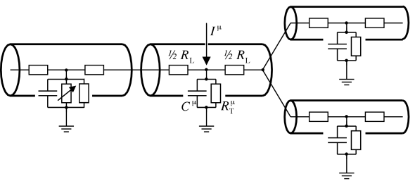
In order to solve for the membrane potential of a complex dendritic tree numerically, compartmental models are used that are the result of the above mentioned discretization. The dendritic tree is divided into small cylindric compartments with an approximatively uniform membrane potential. Each compartment is characterized by its capacity and transversal conductivity. Adjacent compartments are coupled by the longitudinal resistance that are determined by their geometrical properties (cf. Fig. 3.8).
Once numerical methods are used to solve for the membrane potential along the dendritic tree, some or all compartments can be equipped with nonlinear ion channels as well. In this way, effects of nonlinear integration of synaptic input can be studied. Apart from practical problems that arise from a growing complexity of the underlying differential equations, conceptual problems are related to a drastically increasing number of free parameters. To avoid these problems, all nonlinear ion channels responsible for generating spikes are usually lumped together at the soma and the dendritic tree is treated as a passive cable. For a review of the compartmental approach we refer the reader to the book of Bower and Beeman (63). In the following we illustrate the compartmental approach by a model of a pyramidal cell.
Example: A multicompartment model of a deep-layer pyramidal cell
Software tools such as NEURON (90) or GENESIS (63) enable researchers to construct detailed compartmental models of any type of neuron. The morphology of such a detailed model is constrained by the anatomical reconstruction of the corresponding ‘real’ neuron. This is possible if length, size and orientation of each dendritic segment are measured under a microscope, after the neuron has been filled with a suitable dye. Before the anatomical reconstruction, the electrophysiological properties of the neuron can be characterized by stimulating the neuron with a time-dependent electric current. The presence of specific ion channel types can be inferred, with genetic methods, from the composition of the intracellular liquid, extracted from the neuron (514). The distribution of ion channels across the dendrite is probably the least constrained parameter. It is sometimes inferred from another set of experiments on neurons belonging to the same class. All the experimental knowledge about the neuron is then condensed in a computational neuron model. A good example is the model of a deep layer cortical neuron with active dendrites as modeled by Hay et al. [2011].
The complete morphology is divided in 200 compartments, none exceeding 20 m in length. Each compartment has its specific dynamics defined by intra-cellular ionic concentration, transversal ion flux through modelled ion channels, and longitudinal current flux to connected compartments. The membrane capacitance is set to 1 F/cm for the soma and axon and to 2 F/cm in the dendrites to compensate for the presence of dendritic spines. A cocktail of ionic currents is distributed across the different compartments. These are:
-
•
the fast inactivating sodium current (Section 2.2.3 ),
-
•
the persistent sodium current (Section 2.3.3 ),
-
•
the non-specific cation current (Section 2.3.4 ),
-
•
the muscarinic potassium current (Section 2.3.3 ),
-
•
the small conductance calcium-activated potassium current (Section 2.3.4 )
- •
-
•
the high-voltage activated calcium current (mentioned in Section 2.16 ),
- •
-
•
and a calcium pump (Section 2.3.3 ).
In addition, the model contains a slow and a fast inactivating potassium current , , respectively (276).
In the dendrites all these currents are modeled as uniformly distributed except , and . The first one of these, is exponentially distributed along the main dendrite that ascends from the deep layers with low concentration to the top layers with large concentration (272). The two calcium channels were distributed with a uniform distribution in all dendrites except for a single hotspot with a concentration 100 and 10 times higher for and , respectively. Finally, the strength of each ionic current was scaled by choosing the maximal conductance that best fit experimental data.
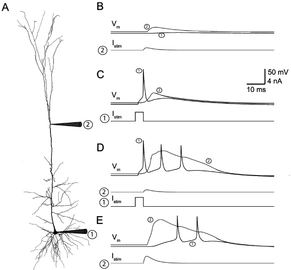
This detailed compartmental model can reproduce quantitatively some features of the deep-layer pyramidal neurons (Fig. 3.9). For example, a small dendritic current injection results in a transient increase of the dendritic voltage, but only a small effect in the soma (Fig. 3.9B). A sufficiently large current pulse in the soma initiates not only a spike at the soma but also a back-propagating action potential travelling into the dendrites (Fig. 3.9C). Note that it is the presence of sodium and potassium currents throughout the dendrites that support the back-propagation. In order to activate the dendritic calcium channels at the hotspot, either a large dendritic injection or a coincidence between the back-propagating action potential and a small dendritic injection is required (Fig. 3.9D-E). The activation of calcium channels in the hotspot introduces a large and long (around 40 ms) depolarizing current that propagates forward to the soma where it eventually causes a burst of action potentials.