4 Dimensionality Reduction and Phase Plane Analysis 4.6 Separation of time scales and reduction to one dimension II Generalized Integrate-and-Fire Neurons

4.7 Summary

The four-dimensional model of Hodgkin-Huxley can be reduced to two dimensions under the assumption that the $m$ -dynamics are fast as compared to $u$ , $h$ , and $n$ , and that the latter two evolve on the same time scale. Two-dimensional models can readily be visualized and studied in the phase plane.

As a first application of phase-plane analysis, we asked whether neuron models have a firing threshold - and found that the answer is something like ‘No, but …’. The answer is ‘No’, because the threshold value depends on the stimulation paradigm. The voltage threshold derived with short current pulses is different from that found with constant current or slow ramps. In type II models the onset of repetitive firing at the rheobase current value starts with nonzero frequency. Type I models exhibit onset of repetitive firing with zero frequency. The transition to repetitive firing in type I models arises through a saddle-node-onto-limit-cycle bifurcation whereas several bifurcation types can give rise to a type II behavior.

The methods of phase plane analysis and dimension reduction are generic tools and will also play a role in several chapters of parts II and IV of this book. In particular, the separation of time scales between the fast voltage variable and the slow recovery variable enables a further reduction of neuronal dynamics to a one-dimensional nonlinear integrate-and-fire model, a fact which we will exploit in the next chapter.

Fig. 4.23: Piecewise linear model with separation of time scale. The inset shows the trajectory (arrows) which follows the $u$ nullcline at a distance of order $\epsilon$ . where $\epsilon\ll 1$ is the ratio of the time scale of the $u$ -dynamics and that of the $w$ -dynamics in unit-free coordinates; see Eq. (4.37).

Literature

An in-depth introduction to dynamical systems, stability of fixed points, and (un)stable manifolds can be found, for example, in the book of Hale and Koçac (204). The book of Strogatz (499) presents the theory of dynamical systems in the context of various problems of physics, chemistry, biology, and engineering. A wealth of applications of dynamical systems to various (mostly non-neuronal) biological systems can be found in the comprehensive book of Murray (355) which also contains a thorough discussion of the FitzHugh-Nagumo model. Phase plane methods applied to neuronal dynamics are discussed in the clearly written review paper of Rinzel and Ermentrout (438) and in the book of Izhikevich (239).

The classification of neuron models as type I and type II can be found in Rinzel and Ermentrout (438) and in Ermentrout (141), and systematically in Izhikevich (239). The steps of dimensionality reduction are presented in Kepler et al. (258).

Exercises

1.

Inhibitory rebound.
a) Draw on the phase plane a schematic representation of the nullclines and flow for the piecewise linear FitzHugh-Nagumo (Eq. 4.36 and Eq. 4.37 ) with parameters $a=c_{1}=-1$ and $b=2$ , and mark the stable fixed point.
b) A hyperpolarizing current is introduced very slowly and increased up to a maximal value of $I=-2$ . Calculate the new value of the stable fixed point. Draw the nullclines and flow for $I=-2$ on a different phase plane.
c) The hyperpolarizing current is suddenly removed. Use the phase planes in a) and b) to find out what will happen. Draw schematically the evolution of the neurons state as a membrane potential time-series and as a trajectory in the phase plane. Use $\epsilon=0.1$ .

Hint: the resting state from b is the initial value of the trajectory in c.
2.

Separation of time scales and quasi-stationary assumption.
a) Consider the following differential equation:

$\tau\frac{dx}{dt}=-x+c,$ (4.38)

where $c$ is a constant. Find the fixed point of this equation. Determine the stability of the fixed point and the solution for any initial condition.
b) Suppose that $c$ is now piecewise constant:

$c=c(t)=\left\{\begin{split}0\;&{\rm for}\,t<0\\ c_{0}\;&{\rm for}\,0\leq t\leq 1\\ 0\;&{\rm for}\,t>1\end{split}\right.$ (4.39)

Calculate the solution $x(t)$ for the initial condition $x(t=-10)=0$ .
c) Now consider the linear system:

$\begin{split}\frac{du}{dt}&=f(u)-m,\\ \end{split}$ (4.40)

$\begin{split} \epsilon\frac{dm}{dt}&=-m+c(u).\\ \end{split}$ (4.41)

Exploit the fact that $\epsilon<<1$ to reduce the system to one equation. Note the similarity with the equations in a) and b).
3.

Separation of time scale and relaxation oscillators.
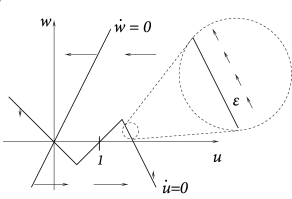
a) Show that in the piecewise linear neuron model defined in Eqs. ( 4.36 ) and ( 4.37 ) the trajectory evolves parallel to the right branch of the $u$ -nullcline, shifted upward by a distance of order $\epsilon$ (Fig. 4.23 ) or parallel to the lifted branch of the $u$ -nullcline, shifted downward by a distance of order $\epsilon$ ).

Hint: If the $u$ -nullcline is given by the function $f(u)$ , set $w(t)=f[u(t)]+\epsilon\,x(t)$ where $x(t)$ is the momentary distance and study the evolution of $du/dt$ and $dw/dt$ according to the differential equations of $u$ and $w$ . At the same time, under the assumption of parallel movement $x(t)$ is a constant and the geometry of the problem in the two-dimensional phase space tells us that $dw/dt=(df/du)\,(du/dt)$ . Show that this leads to a consistent solution for the distance $x$ .
b) What is the time course of the voltage $u(t)$ while the trajectory follows the branch?